Ensemble Clustering - a cluster analysis tool for climate model simulations (EnsClus)#
Overview#
EnsClus is a cluster analysis tool in Python, based on the k-means algorithm, for ensembles of climate model simulations.
Multi-model studies allow to investigate climate processes beyond the limitations of individual models by means of inter-comparison or averages of several members of an ensemble. With large ensembles, it is often an advantage to be able to group members according to similar characteristics and to select the most representative member for each cluster.
The user chooses which feature of the data is used to group the ensemble members by clustering: time mean, maximum, a certain percentile (e.g., 75% as in the examples below), standard deviation and trend over the time period. For each ensemble member this value is computed at each grid point, obtaining N lat-lon maps, where N is the number of ensemble members. The anomaly is computed subtracting the ensemble mean of these maps to each of the single maps. The anomaly is therefore computed with respect to the ensemble members (and not with respect to the time) and the Empirical Orthogonal Function (EOF) analysis is applied to these anomaly maps.
Regarding the EOF analysis, the user can choose either how many Principal Components (PCs) to retain or the percentage of explained variance to keep. After reducing dimensionality via EOF analysis, k-means analysis is applied using the desired subset of PCs.
The major final outputs are the classification in clusters, i.e. which member belongs to which cluster (in k-means analysis the number k of clusters needs to be defined prior to the analysis) and the most representative member for each cluster, which is the closest member to the cluster centroid.
Other outputs refer to the statistics of clustering: in the PC space, the minimum and the maximum distance between a member in a cluster and the cluster centroid (i.e. the closest and the furthest member), the intra-cluster standard deviation for each cluster (i.e. how much the cluster is compact).
Available recipes and diagnostics#
Recipes are stored in recipes/
recipe_ensclus.yml
Diagnostics are stored in diag_scripts/ensclus/
ensclus.py
and subroutines
ens_anom.py
ens_eof_kmeans.py
ens_plots.py
eof_tool.py
read_netcdf.py
sel_season_area.py
User settings#
Required settings for script
season: season over which to perform seasonal averaging (DJF, DJFM, NDJFM, JJA)
area: region of interest (EAT=Euro-Atlantic, PNA=Pacific North American, NH=Northern Hemisphere, EU=Europe)
extreme: extreme to consider: XXth_percentile (XX can be set arbitrarily, e.g. 75th_percentile), mean (mean value over the period), maximum (maximum value over the period), std (standard deviation), trend (linear trend over the period)
numclus: number of clusters to be computed
perc: percentage of variance to be explained by PCs (select either this or numpcs, default=80)
numpcs: number of PCs to retain (has priority over perc unless it is set to 0 (default))
Optional settings for script
max_plot_panels: maximum number of panels (datasets) in a plot. When exceeded multiple plots are created. Default: 72
Variables#
chosen by user (e.g., precipitation as in the example)
Observations and reformat scripts#
None.
References#
Straus, D. M., S. Corti, and F. Molteni: Circulation regimes: Chaotic variability vs. SST forced predictability. J. Climate, 20, 2251–2272, 2007. https://doi.org/10.1175/JCLI4070.1
Example plots#
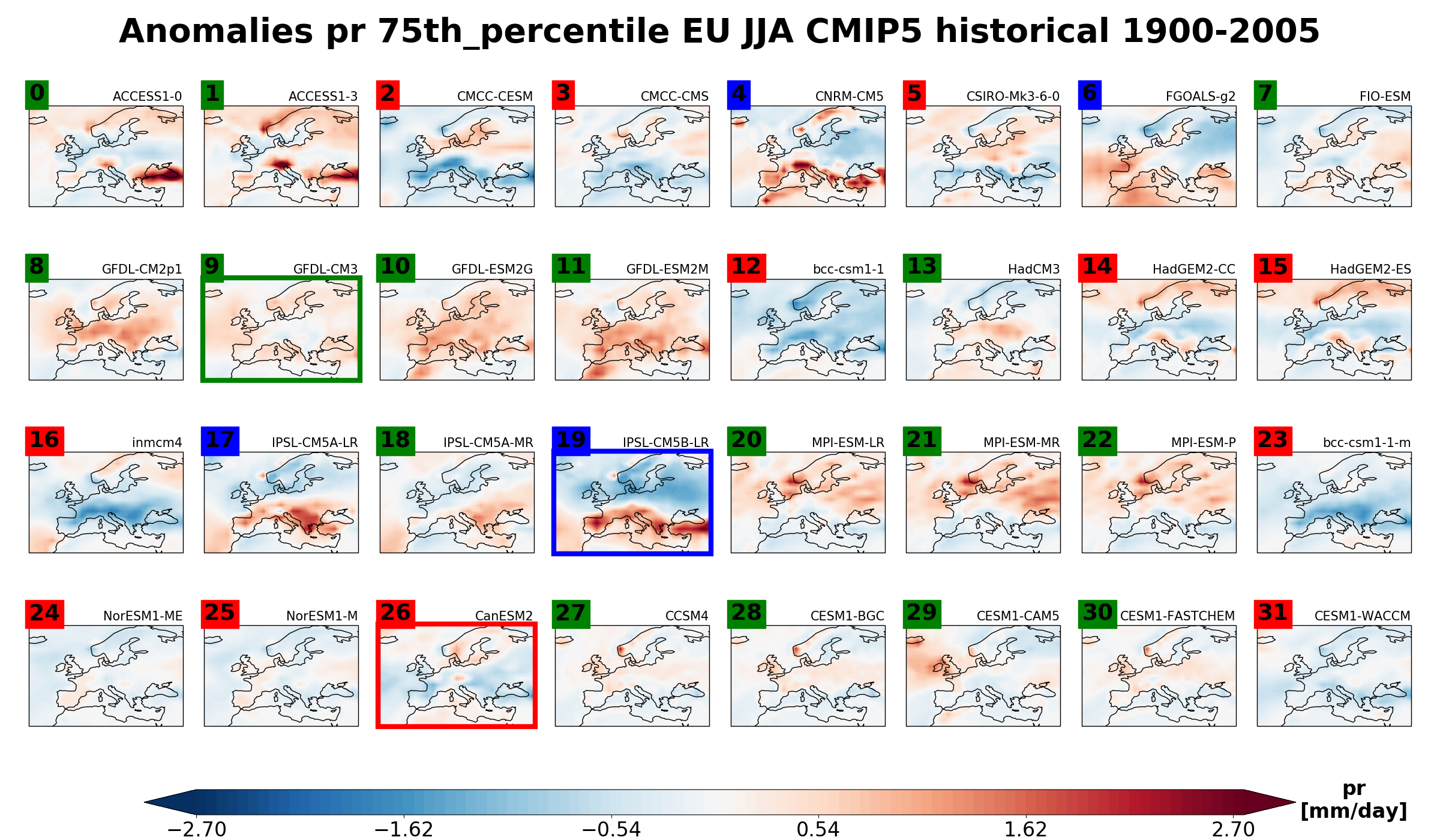
Fig. 380 Clustering based on the 75th percentile of historical summer (JJA) precipitation rate for CMIP5 models over 1900-2005. 3 clusters are computed, based on the principal components explaining 80% of the variance. The 32 models are grouped in three different clusters. The green cluster is the most populated with 16 ensemble members mostly characterized by a positive anomaly over central-north Europe. The red cluster counts 12 elements that exhibit a negative anomaly centered over southern Europe. The third cluster – labelled in blue- includes only 4 models showing a north-south dipolar precipitation anomaly, with a wetter than average Mediterranean counteracting dryer North-Europe. Ensemble members No.9, No.26 and No.19 are the “specimen” of each cluster, i.e. the model simulations that better represent the main features of that cluster. These ensemble members can eventually be used as representative of the whole possible outcomes of the multi-model ensemble distribution associated to the 32 CMIP5 historical integrations for the summer precipitation rate 75 th percentile over Europe when these outcomes are reduced from 32 to 3. The number of ensemble members of each cluster might provide a measure of the probability of occurrence of each cluster.#