Evaluate water vapor short wave radiance absorption schemes of ESMs with the observations, including ESACCI data.

Overview

The recipe contains several diagnostics to use ESACCI water vapour data to evaluate CMIP models.

The diagnostic deangelisf3f4.py reproduces figures 3 and 4 from DeAngelis et al. (2015): See also doc/sphinx/source/recipes/recipe_deangelis15nat.rst This paper compares models with different schemes for water vapor short wave radiance absorption with the observations. Schemes using pseudo-k-distributions with more than 20 exponential terms show the best results.

The diagnostic diag_tropopause.py plots given variable at cold point tropopause height, here Specific Humidity (hus) is used. This will be calculated from the ESACCI water vapour data CDR-4, which are planed to consist of three-dimensional vertically resolved monthly mean water vapour data (in ppmv) with spatial resolution of 100 km, covering the troposphere and lower stratosphere. The envisaged coverage is 2010-2014. The calculation of hus from water vapour in ppmv will be part of the cmorizer. Here, ERA-Interim data are used.

The diagnostic diag_tropopause_zonalmean.py plots zonal mean for given variable for all pressure levels between 250 and 1hPa and at cold point tropopause height. Here Specific Humidity (hus) is used. This will be calculated from the ESACCI water vapour data CDR-3, which are planed to contain the vertically resolved water vapour ECV in units of ppmv (volume mixing ratio) and will be provided as zonal monthly means on the SPARC Data Initiative latitude/pressure level grid (SPARC, 2017; Hegglin et al., 2013). It covers the vertical range between 250 hPa and 1 hPa, and the time period 1985 to the end of 2019. The calculation of hus from water vapour in ppmv will be part of the cmorizer. Here, ERA-Interim data are used.

Available recipes and diagnostics

Recipes are stored in recipes/

• recipe_cmug_h2o.yml

Diagnostics are stored in diag_scripts/

• deangelis15nat/deangelisf3f4.py

• cmug_h2o/diag_tropopause.py

• cmug_h2o/diag_tropopause_zonalmean.py

User settings in recipe

The recipe can be run with different CMIP5 and CMIP6 models.

deangelisf3f4.py: For each model, two experiments must be given: a pre industrial control run, and a scenario with 4 times CO₂. Possibly, 150 years should be given, but shorter time series work as well. Currently, HOAPS data are included as place holder for expected ESACCI-WV data, type CDR-2: Gridded monthly time series of TCWV in units of kg/m2 (corresponds to prw) that cover the global land and ocean areas with a spatial resolution of 0.05° / 0.5° for the period July 2002 to December 2017.

Variables

deangelisf3f4.py: * rsnstcs (atmos, monthly, longitude, latitude, time) * rsnstcsnorm (atmos, monthly, longitude, latitude, time) * prw (atmos, monthly, longitude, latitude, time) * tas (atmos, monthly, longitude, latitude, time)

diag_tropopause.py: * hus (atmos, monthly, longitude, latitude, time, plev) * ta (atmos, monthly, longitude, latitude, time, plev)

diag_tropopause_zonalmean.py: * hus (atmos, monthly, longitude, latitude, time, plev) * ta (atmos, monthly, longitude, latitude, time, plev)

Observations and reformat scripts

deangelisf3f4.py:

• rsnstcs:

  CERES-EBAF

• prw

  HOAPS, planed for ESACCI-WV data, type CDR-2

diag_tropopause.py:

• hus

  ERA-Interim, ESACCI water vapour paned

diag_tropopause_zonalmean.py:

• hus

  ERA-Interim, ESACCI water vapour paned

References

• DeAngelis, A. M., Qu, X., Zelinka, M. D., and Hall, A.: An observational radiative constraint on hydrologic cycle intensification, Nature, 528, 249, 2015.

Example plots

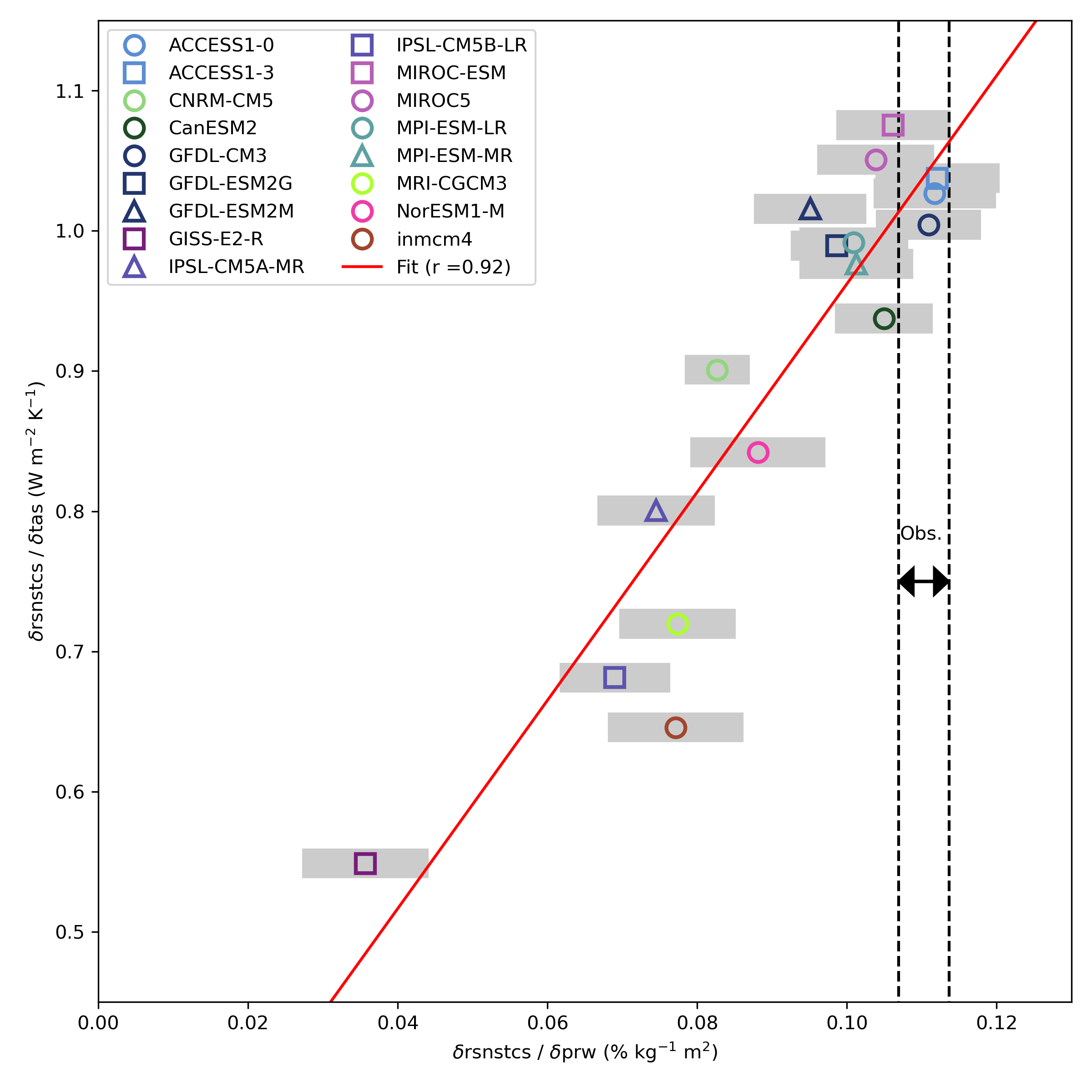
Fig. 16 Scatter plot and regression line computed between the ratio of the change of net short wave radiation (rsnst) and the change of the Water Vapor Path (prw) against the ratio of the change of netshort wave radiation for clear skye (rsnstcs) and the the change of surface temperature (tas). The width of horizontal shading for models and the vertical dashed lines for observations (Obs.) represent statistical uncertainties of the ratio, as the 95% confidence interval (CI) of the regression slope to the rsnst versus prw curve. For the prw observations ESACCI CDR-2 data from 2003 to 2014 are used.

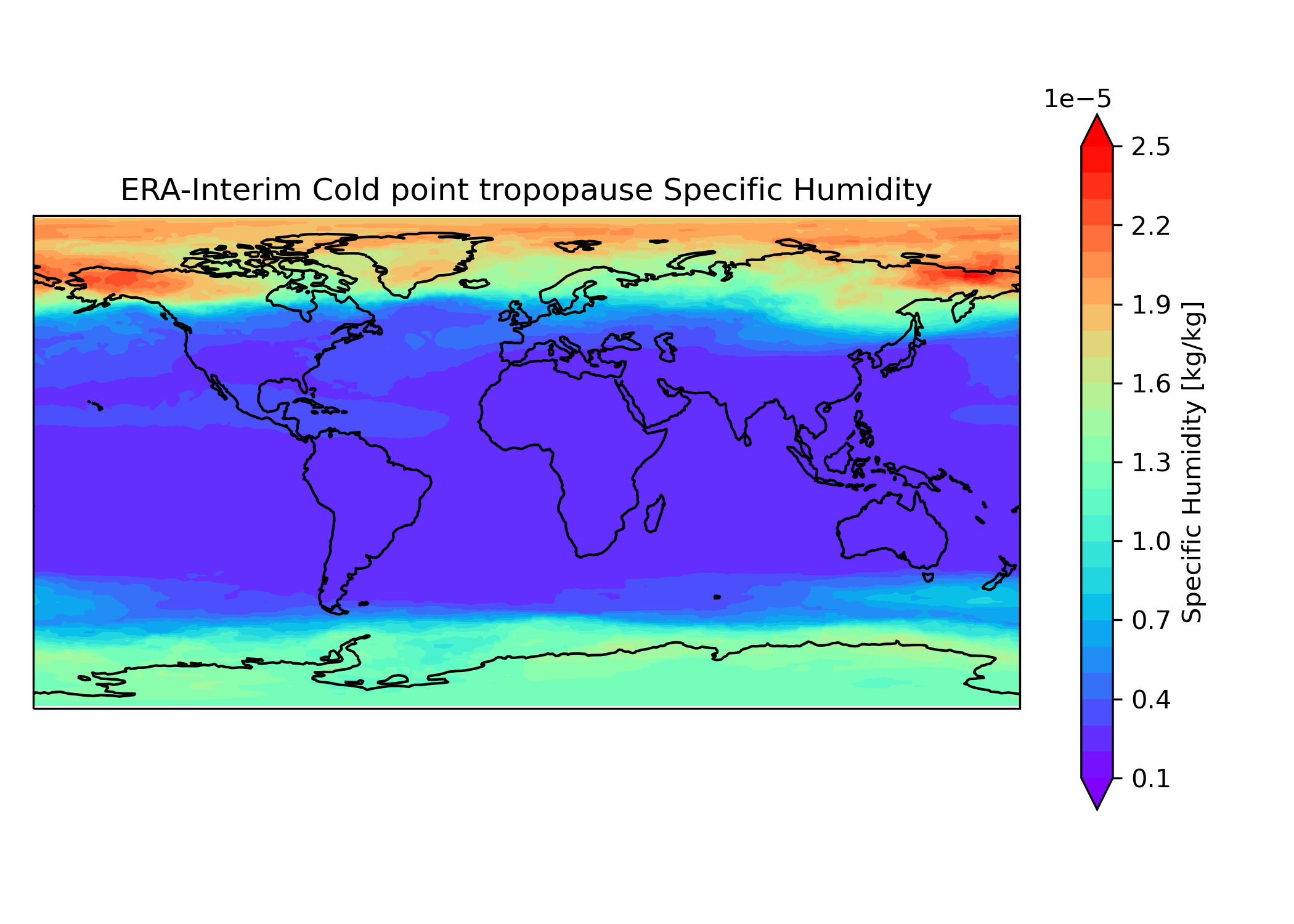
Fig. 17 Map of the average Specific Humidity (hus) at the cold point tropopause from ERA-Interim data. The diagnostic averages the complete time series, here 2010-2014.

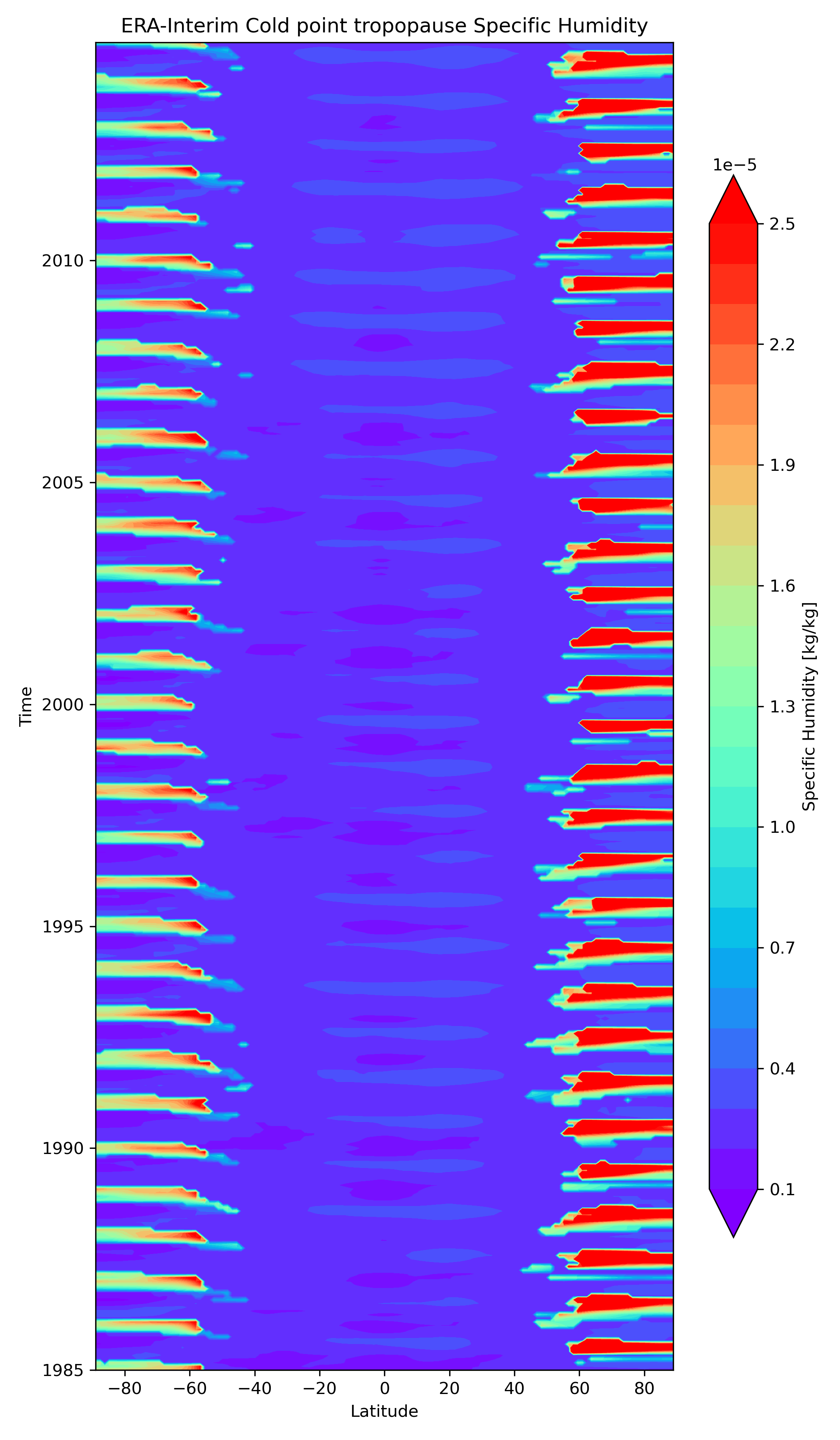
Fig. 18 Latitude versus time plot of the Specific Humidity (hus) at the cold point tropopause from ERA-Interim data.

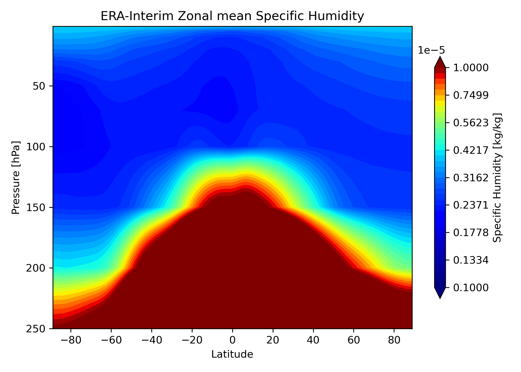
Fig. 19 Zonal average Specific Humidity (hus) between 250 and 1 hPa from ERA-Interim data. The diagnostic averages the complete time series, here 1985-2014.

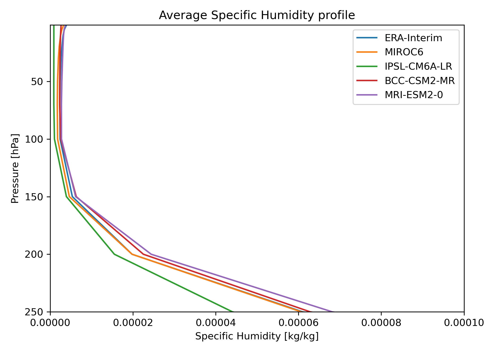
Fig. 20 Average Specific Humidity (hus) profile between 250 and 1 hPa from ERA-Interim and CMIP6 model data. The diagnostic averages the complete time series, here 1985-2014.