IPCC AR5 Chapter 9 (selected figures)

Overview

The goal of this recipe is to collect diagnostics to reproduce Chapter 9 of AR5, so that the plots can be readily reproduced and compared to previous CMIP versions. In this way we can next time start with what was available in the previous round and can focus on developing more innovative methods of analysis rather than constantly having to “re-invent the wheel”.

Note

Please note that most recipes have been modified to include only models that are (still) readily available via ESGF. Plots produced may therefore look different than the original figures from IPCC AR5.

The plots are produced collecting the diagnostics from individual recipes. The following figures from Flato et al. (2013) can currently be reproduced:

• Figure 9.2 a,b,c: Annual-mean surface air temperature for the period 1980-2005. a) multi-model mean, b) bias as the difference between the CMIP5 multi-model mean and the climatology from ERA-Interim (Dee et al., 2011), c) mean absolute model error with respect to the climatology from ERA-Interim.

• Figure 9.3: Seasonality (December-January-February minus June-July-August) of surface (2 m) air temperature (°C) for the period 1980-2005. (a) Multi-model mean for the historical experiment. (b) Multi-model mean of absolute seasonality. (c) Difference between the multi-model mean and the ERA-Interim reanalysis seasonality. (d) Difference between the multi-model mean and the ERA-Interim absolute seasonality.

• Figure 9.4: Annual-mean precipitation rate (mm day-1) for the period 1980-2005. a) multi-model mean, b) bias as the difference between the CMIP5 multi-model mean and the climatology from the Global Precipitation Climatology Project (Adler et al., 2003), c) multi-model mean absolute error with respect to observations, and d) multi-model mean error relative to the multi-model mean precipitation itself.

• Figure 9.5: Climatological (1985-2005) annual-mean cloud radiative effects in Wm-2 for the CMIP5 models against CERES EBAF (2001-2011) in Wm-2. Top row shows the shortwave effect; middle row the longwave effect, and bottom row the net effect. Multi-model-mean biases against CERES EBAF 2.6 are shown on the left, whereas the right panels show zonal averages from CERES EBAF 2.6 (black), the individual CMIP5 models (thin gray lines), and the multi-model mean (thick red line).

• Figure 9.6: Centered pattern correlations between models and observations for the annual mean climatology over the period 1980–1999. Results are shown for individual CMIP3 (black) and CMIP5 (blue) models as thin dashes, along with the corresponding ensemble average (thick dash) and median (open circle). The four variables shown are surface air temperature (TAS), top of the atmosphere (TOA) outgoing longwave radiation (RLUT), precipitation (PR) and TOA shortwave cloud radiative effect (SW CRE). The correlations between the reference and alternate observations are also shown (solid green circles).

• Figure 9.8: Observed and simulated time series of the anomalies in annual and global mean surface temperature. All anomalies are differences from the 1961-1990 time-mean of each individual time series. The reference period 1961-1990 is indicated by yellow shading; vertical dashed grey lines represent times of major volcanic eruptions. Single simulations for CMIP5 models (thin lines); multi-model mean (thick red line); different observations (thick black lines). Dataset pre-processing like described in Jones et al., 2013.

• Figure 9.14: Sea surface temperature plots for zonal mean error, equatorial (5 deg north to 5 deg south) mean error, and multi model mean for zonal error and equatorial mean.

• Figure 9.24: Time series of (a) Arctic and (b) Antarctic sea ice extent; trend distributions of (c) September Arctic and (d) February Antarctic sea ice extent.

• Figure 9.26: Ensemble-mean global ocean carbon uptake (a) and global land carbon uptake (b) in the CMIP5 ESMs for the historical period 1900–2005. For comparison, the observation-based estimates provided by the Global Carbon Project (GCP) are also shown (thick black line). The confidence limits on the ensemble mean are derived by assuming that the CMIP5 models are drawn from a t-distribution. The grey areas show the range of annual mean fluxes simulated across the model ensemble. This figure includes results from all CMIP5 models that reported land CO2 fluxes, ocean CO2 fluxes, or both (Anav et al., 2013).

• Figure 9.27: Simulation of global mean (a) atmosphere–ocean CO2 fluxes (“fgCO2”) and (b) net atmosphere–land CO2 fluxes (“NBP”), by ESMs for the period 1986–2005. For comparison, the observation-based estimates provided by Global Carbon Project (GCP) and the Japanese Meteorological Agency (JMA) atmospheric inversion are also shown. The error bars for the ESMs and observations represent interannual variability in the fluxes, calculated as the standard deviation of the annual means over the period 1986–2005.

• Figure 9.38: Seasonal cycle for the surface temperature or precipitation over land within defined regions multi-model mean and difference to reference dataset or absolute annual cycle can be chosen.

• Figure 9.39: Seasonal bias box and whiskers plot for surface temperature or precipitation within SREX (IPCC Special Report on Managing the Risks of Extreme Events and Disasters to Advance Climate Change Adaptation) regions.

• Figure 9.40: Seasonal bias box and whiskers plot for surface temperature or precipitation within defined polar and ocean regions.

• Figure 9.41b: Comparison between observations and models for variable values within defined regions.

• Figure 9.42a: Equilibrium climate sensitivity (ECS) against the global mean surface air temperature, both for the period 1961-1990 and for the pre-industrial control runs.

• Figure 9.42b: Transient climate response (TCR) against equilibrium climate sensitivity (ECS).

• Figure 9.45a: Scatterplot of springtime snow-albedo effect values in climate change vs. springtime d(alpha_s)/d(T_s) values in the seasonal cycle in transient climate change experiments (Hall and Qu, 2006).

Available recipes and diagnostics

Recipes are stored in esmvaltool/recipes/recipe_ipccwg1ar5ch9

• recipe_flato13ipcc_figures_92_95.yml: Figures 9.2, 9.3, 9.4, 9.5

• recipe_flato13ipcc_figure_96.yml: Figure 9.6

• recipe_flato13ipcc_figure_98.yml: Figure 9.8

• recipe_flato13ipcc_figure_914.yml: Figure 9.14

• recipe_flato13ipcc_figure_924.yml: Figure 9.24

• recipe_flato13ipcc_figures_926_927.yml: Figures 9.26 and 9.27

• recipe_flato13ipcc_figure_942.yml: Figure 9.42

• recipe_flato13ipcc_figure_945a.yml: Figure 9.45a

• recipe_flato13ipcc_figures_938_941_cmip3.yml: Figures 9.38, 9.39, 9.40, and 9.41

• recipe_flato13ipcc_figures_938_941_cmip6.yml: Figures 9.38, 9.39, 9.40, and 9.41 CMIP6 instead of CMIP3

• recipe_weigel21gmd_figures_13_16.yml: ESMValTool paper version (Weigel et al., 2021) of Figures 9.38, 9.39, 9.40, and 9.41, only CMIP5

Diagnostics are stored in esmvaltool/diag_scripts/

• carbon_cycle/main.ncl: See here.

• climate_metrics/ecs.py: See here.

• clouds/clouds_bias.ncl: global maps of the multi-model mean and the multi-model mean bias (Fig. 9.2, 9.4)

• clouds/clouds_ipcc.ncl: global maps of multi-model mean minus observations + zonal averages of individual models, multi-model mean and observations (Fig. 9.5)

• ipcc_ar5/ch09_fig09_3.ncl: multi-model mean seasonality of near-surface temperature (Fig. 9.3)

• ipcc_ar5/ch09_fig09_6.ncl: calculating pattern correlations of annual mean climatologies for one variable (Fig 9.6 preprocessing)

• ipcc_ar5/ch09_fig09_6_collect.ncl: collecting pattern correlation for each variable and plotting correlation plot (Fig 9.6)

• ipcc_ar5/tsline.ncl: time series of the global mean (anomaly) (Fig. 9.8)

• ipcc_ar5/ch09_fig09_14.py: Zonally averaged and equatorial SST (Fig. 9.14)

• seaice/seaice_tsline.ncl: Time series of sea ice extent (Fig. 9.24a/b)

• seaice/seaice_trends.ncl: Trend distributions of sea ice extent (Fig 9.24c/d)

• regional_downscaling/Figure9_38.ncl (Fig 9.38a (variable tas) and Fig 9.38b (variable pr))

• regional_downscaling/Figure9_39.ncl (Fig 9.39a/c/e (variable tas) and Fig 9.39b/d/f (variable pr))

• regional_downscaling/Figure9_40.ncl (Fig 9.40a/c/e (variable tas) and Fig 9.40b/d/f (variable pr))

• regional_downscaling/Figure9_41.ncl (Fig 9.41b)

• ipcc_ar5/ch09_fig09_42a.py: ECS vs. surface air temperature (Fig. 9.42a)

• ipcc_ar5/ch09_fig09_42b.py: TCR vs. ECS (Fig. 9.42b)

• emergent_constraints/snowalbedo.ncl: snow-albedo effect (Fig. 9.45a)

User settings in recipe

1. Script carbon_cycle/main.ncl

   See here.

2. Script climate_metrics/ecs.py

   See here.

3. Script clouds/clouds_bias.ncl

   Required settings (scripts)

   none

   Optional settings (scripts)

   • plot_abs_diff: additionally also plot absolute differences (true, false)

   • plot_rel_diff: additionally also plot relative differences (true, false)

   • projection: map projection, e.g., Mollweide, Mercator

   • timemean: time averaging, i.e. “seasonalclim” (DJF, MAM, JJA, SON), “annualclim” (annual mean)

   • Required settings (variables)*

   • reference_dataset: name of reference dataset

   Optional settings (variables)

   • long_name: description of variable

   Color tables

   • variable “tas”: diag_scripts/shared/plot/rgb/ipcc-tas.rgb, diag_scripts/shared/plot/rgb/ipcc-tas-delta.rgb

   • variable “pr-mmday”: diag_scripts/shared/plots/rgb/ipcc-precip.rgb, diag_scripts/shared/plot/rgb/ipcc-precip-delta.rgb

4. Script clouds/clouds_ipcc.ncl

   Required settings (scripts)

   none

   Optional settings (scripts)

   • explicit_cn_levels: contour levels

   • mask_ts_sea_ice: true = mask T < 272 K as sea ice (only for variable “ts”); false = no additional grid cells masked for variable “ts”

   • projection: map projection, e.g., Mollweide, Mercator

   • styleset: style set for zonal mean plot (“CMIP5”, “DEFAULT”)

   • timemean: time averaging, i.e. “seasonalclim” (DJF, MAM, JJA, SON), “annualclim” (annual mean)

   • valid_fraction: used for creating sea ice mask (mask_ts_sea_ice = true): fraction of valid time steps required to mask grid cell as valid data

   Required settings (variables)

   • reference_dataset: name of reference data set

   Optional settings (variables)

   • long_name: description of variable

   • units: variable units

   Color tables

   • variables “pr”, “pr-mmday”: diag_scripts/shared/plot/rgb/ipcc-precip-delta.rgb

5. Script ipcc_ar5/tsline.ncl

   Required settings for script

   • styleset: as in diag_scripts/shared/plot/style.ncl functions

   Optional settings for script

   • time_avg: type of time average (currently only “yearly” and “monthly” are available).

   • ts_anomaly: calculates anomalies with respect to the defined period; for each grid point by removing the mean for the given calendar month (requiring at least 50% of the data to be non-missing)

   • ref_start: start year of reference period for anomalies

   • ref_end: end year of reference period for anomalies

   • ref_value: if true, right panel with mean values is attached

   • ref_mask: if true, model fields will be masked by reference fields

   • region: name of domain

   • plot_units: variable unit for plotting

   • y-min: set min of y-axis

   • y-max: set max of y-axis

   • mean_nh_sh: if true, calculate first NH and SH mean

   • volcanoes: if true, lines of main volcanic eruptions will be added

   • run_ave: if not equal 0 than calculate running mean over this number of years

   • header: if true, region name as header

   Required settings for variables

   none

   Optional settings for variables

   • reference_dataset: reference dataset; REQUIRED when calculating anomalies

   Color tables

   • e.g. diag_scripts/shared/plot/styles/cmip5.style

6. Script ipcc_ar5/ch09_fig09_3.ncl

   Required settings for script

   none

   Optional settings for script

   • projection: map projection, e.g., Mollweide, Mercator (default = Robinson)

   Required settings for variables

   • reference_dataset: name of reference observation

   Optional settings for variables

   • map_diff_levels: explicit contour levels for plotting

7. Script ipcc_ar5/ch09_fig09_6.ncl

   Required settings for variables

   • reference_dataset: name of reference observation

   Optional settings for variables

   • alternative_dataset: name of alternative observations

8. Script ipcc_ar5/ch09_fig09_6_collect.ncl

   Required settings for script

   none

   Optional settings for script

   • diag_order: List of diagnostic names in the order variables should appear on x-axis

9. Script seaice/seaice_trends.ncl

   Required settings (scripts)

   • month: selected month (1, 2, …, 12) or annual mean (“A”)

   • region: region to be analyzed ( “Arctic” or “Antarctic”)

   Optional settings (scripts)

   • fill_pole_hole: fill observational hole at North pole, Default: False

   Optional settings (variables)

   • ref_model: array of references plotted as vertical lines

10. Script seaice/seaice_tsline.ncl

    Required settings (scripts)

    • region: Arctic, Antarctic

    • month: annual mean (A), or month number (3 = March, for Antarctic; 9 = September for Arctic)

    Optional settings (scripts)

    • styleset: for plot_type cycle only (cmip5, cmip6, default)

    • multi_model_mean: plot multi-model mean and standard deviation (default: False)

    • EMs_in_lg: create a legend label for individual ensemble members (default: False)

    • fill_pole_hole: fill polar hole (typically in satellite data) with sic = 1 (default: False)

11. Script regional_downscaling/Figure9.38.ncl

    Required settings for script

    none

    Optional settings (scripts)

    • styleset: for plot_type cycle (e.g. CMIP5, CMIP6), default “CMIP5”

    • fig938_region_label: Labels for regions, which should be included ([“WNA”, “ENA”, “CAM”, “TSA”, “SSA”, “EUM”, “NAF”,”CAF”, “SAF”, “NAS”, “CAS”, “EAS”, “SAS”, “SEA”, “AUS”]), default “WNA”

    • fig938_project_MMM: projects to average, default “CMIP5”

    • fig938_experiment_MMM: experiments to average, default “historical”

    • fig938_mip_MMM: mip to average, default “Amon”

    • fig938_names_MMM: names in legend i.e. ([“CMIP5”,”CMIP3”]), default fig938_project_MMM

    • fig938_colors_MMM: Color for multi-model mean (e.g. [“red”]), default “red”

    • If set fig938_mip_MMM, fig938_experiment_MMM, fig938_project_MMM, fig938_names_MMM, and fig938_colors_MMM must have the same number of elements

    • fig938_refModel: Reference data set for differences default “ERA-Interim”

    • fig938_MMM: Plot multi-model mean (true/false), default “true”

    • fig938_YMin: minimum Y Axis

    • fig938_YMax: maximum Y Axis

    • fig938_diff: Difference to reference data (true) or absolute annual cycle (false), default “true”

12. Script regional_downscaling/Figure9.39.ncl

    Required settings (scripts)

    • reference_dataset: reference dataset name (set of variables)

    Optional settings (scripts)

    • styleset: for plot_type cycle (e.g. CMIP5, CMIP6), default “CMIP5”

    • fig939_season: seasons i.e. ([“DJF”,”JJA”,”ANN”]), default “DJF”

    • fig939_region_label: Labels for regions, which should be included ([“ALAs”,”CGIs”,”WNAs”,”CNAs”,”ENAs”,”CAMs”,”AMZs”,”NEBs”,”WSAs”,”SSAs”, “NEUs”,”CEUs”,”MEDs”,”SAHs”,”WAFs”,”EAFs”,”SAFs”,”NASs”,”WASs”,”CASs”, “TIBs”,”EASs”,”SASs”,”SEAs”,”NAUs”,”SAUs”]), default “ALAs”

    • fig939_project_MMM: projects to average, default “CMIP5”

    • fig939_experiment_MMM: experiments to average, default “historical”

    • fig939_mip_MMM: mip to average, default “Amon”

    • fig939_MMM: Plot multi-model mean (true/false)

    • fig939_names_MMM: names in legend i.e. ([“CMIP5”,”CMIP3”])

    • fig939_YMin: minimum Y Axis

    • fig939_YMax: maximum Y Axis

    • fig939_vert_line_pos: i.e. ([6,10,13,17,24,26])

    • fig939_vert_line_label: labels of vertical lines, i.e. ([“North America”, “South America”,”Europe”,”Africa”,”Asia”,”Australia”])

    • fig939_mode: True= cumulative mode

13. Script regional_downscaling/Figure9.40.ncl

    Required settings (scripts)

    • reference_dataset: reference dataset name (set of variables)

    Optional settings (scripts)

    • styleset: for plot_type cycle (e.g. CMIP5, CMIP6), default “CMIP5”

    • fig940_season: seasons i.e. ([“DJF”,”JJA”,”ANN”]), default “DJF”

    • fig940_region_label: Labels for regions, which should be included ([“Arctic_land”,”Arctic_sea”,”Antarctic_land”,”Antarctic_sea”, “Caribbean”,”WesternIndianOcean”,”NorthernIndianOcean”, “NorthernTropicalPacific”,”EquatorialTropicalPacific”, “SouthernTropicalPacific”,”World_land”,”World_sea”,”World”]), default “Arctic_land”

    • fig940_project_MMM: projects to average, default “CMIP5”

    • fig940_experiment_MMM: experiments to average, default “historical”

    • fig940_mip_MMM: mip to average, default “Amon”

    • fig940_MMM: Plot multi-model mean (true/false)

    • fig940_names_MMM: names in legend i.e. ([“CMIP5”,”CMIP3”])

    • fig940_YMin: minimum Y Axis

    • fig940_YMax: maximum Y Axis

    • fig940_vert_line_pos: i.e. ([6,10,13,17,24,26])

    • fig940_vert_line_label: labels of vertical lines, i.e. ([“North America”, “South America”,”Europe”,”Africa”,”Asia”,”Australia”])

    • fig940_mode: True= cumulative mode

14. Script regional_downscaling/Figure9.41.ncl

    Required settings (scripts)

    • reference_dataset: reference dataset name (set of variables)

    Optional settings (scripts)

    • styleset: for plot_type cycle (e.g. CMIP5, CMIP6), default “CMIP5”

    • fig941_region_label: Labels for regions, which should be included ([“ALAs”,”CGIs”,”WNAs”,”CNAs”,”ENAs”,”CAMs”,”AMZs”,”NEBs”,”WSAs”,”SSAs”, “NEUs”,”CEUs”,”MEDs”,”SAHs”,”WAFs”,”EAFs”,”SAFs”,”NASs”,”WASs”,”CASs”, “TIBs”,”EASs”,”SASs”,”SEAs”,”NAUs”,”SAUs”]), default “MEDs”

15. Script ipcc_ar5/ch09_fig09_42a.py

    Required settings for script

    none

    Optional settings for script

    • axes_functions: dict containing methods executed for the plot’s matplotlib.axes.Axes object.

    • dataset_style: name of the style file (located in esmvaltool.diag_scripts.shared.plot.styles_python).

    • matplotlib_style: name of the matplotlib style file (located in esmvaltool.diag_scripts.shared.plot.styles_python.matplotlib).

    • save: dict containing keyword arguments for the function matplotlib.pyplot.savefig().

    • seaborn_settings: Options for seaborn.set_theme() (affects all plots).

1. Script ipcc_ar5/ch09_fig09_42b.py

   Required settings for script

   none

   Optional settings for script

   • dataset_style: Dataset style file (located in esmvaltool.diag_scripts.shared.plot.styles_python). The entry marker is ignored when marker_file is given.

   • log_x: Apply logarithm to X axis (ECS).

   • log_y: Apply logarithm to Y axis (TCR).

   • marker_column: Name of the column to look up markers in marker_file.

   • marker_file: CSV file with markers (can also be integers). Must have the columns dataset and marker (or the column specified by marker_column). If a relative path is given, assumes that this is a pattern to search for ancestor files.

   • savefig_kwargs: Keyword arguments for matplotlib.pyplot.savefig().

   • seaborn_settings: Options for seaborn.set_theme() (affects all plots).

   • x_lim: Plot limits for X axis (ECS).

   • y_lim: Plot limits for Y axis (TCR).

2. Script emergent_constraints/snowalbedo.ncl

   Required settings for script

   • exp_presentday: name of present-day experiment (e.g. “historical”)

   • exp_future: name of climate change experiment (e.g. “rcp45”)

   Optional settings for script

   • diagminmax: observational uncertainty (min and max)

   • legend_outside: create extra file with legend (true, false)

   • styleset: e.g. “CMIP5” (if not set, this diagnostic will create its own color table and symbols for plotting)

   • suffix: string to be added to output filenames

   • xmax: upper limit of x-axis (default = automatic)

   • xmin: lower limit of x-axis (default = automatic)

   • ymax: upper limit of y-axis (default = automatic)

   • ymin: lower limit of y-axis (default = automatic)

   Required settings for variables

   • ref_model: name of reference data set

   Optional settings for variables

   none

Variables

• areacello (fx, longitude latitude)

• fgco2 (ocean, monthly mean, longitude latitude time)

• nbp (ocean, monthly mean, longitude latitude time)

• pr (atmos, monthly mean, longitude latitude time)

• rlut, rlutcs (atmos, monthly mean, longitude latitude time)

• rsdt (atmos, monthly mean, longitude latitude time)

• rsuscs, rsdscs (atmos, monthly mean, longitude latitude time)

• rsut, rsutcs (atmos, monthly mean, longitude latitude time)

• sic (ocean-ice, monthly mean, longitude latitude time)

• tas (atmos, monthly mean, longitude latitude time)

• tos (ocean, monthly mean, longitude, latitude, time)

Observations and reformat scripts

Note: (1) obs4MIPs data can be used directly without any preprocessing; (2) see headers of reformat scripts for non-obs4MIPs data for download instructions.

• CERES-EBAF (rlut, rlutcs, rsut, rsutcs - obs4MIPs)

• ERA-Interim (tas, ta, ua, va, zg, hus - esmvaltool/cmorizers/data/formatters/datasets/era-interim.py)

• GCP2018 (fgco2, nbp - esmvaltool/cmorizers/data/formatters/datasets/gcp2018.py)

• GPCP-SG (pr - obs4MIPs)

• JMA-TRANSCOM (fgco2, nbp - esmvaltool/cmorizers/data/formatters/datasets/jma_transcom.py)

• HadCRUT4 (tas - esmvaltool/cmorizers/data/formatters/datasets/hadcrut4.ncl)

• HadISST (sic, tos - esmvaltool/cmorizers/data/formatters/datasets/hadisst.ncl)

• ISCCP-FH (rsuscs, rsdscs, rsdt - esmvaltool/cmorizers/data/formatters/datasets/isccp_fh.ncl)

References

• Flato, G., J. Marotzke, B. Abiodun, P. Braconnot, S.C. Chou, W. Collins, P. Cox, F. Driouech, S. Emori, V. Eyring, C. Forest, P. Gleckler, E. Guilyardi, C. Jakob, V. Kattsov, C. Reason and M. Rummukainen, 2013: Evaluation of Climate Models. In: Climate Change 2013: The Physical Science Basis. Contribution of Working Group I to the Fifth Assessment Report of the Intergovernmental Panel on Climate Change [Stocker, T.F., D. Qin, G.-K. Plattner, M. Tignor, S.K. Allen, J. Boschung, A. Nauels, Y. Xia, V. Bex and P.M. Midgley (eds.)]. Cambridge University Press, Cambridge, United Kingdom and New York, NY, USA.

• Hall, A., and X. Qu, 2006: Using the current seasonal cycle to constrain snow albedo feedback in future climate change, Geophys. Res. Lett., 33, L03502, doi:10.1029/2005GL025127.

• Jones et al., 2013: Attribution of observed historical near-surface temperature variations to anthropogenic and natural causes using CMIP5 simulations. Journal of Geophysical Research: Atmosphere, 118, 4001-4024, doi:10.1002/jgrd.50239.

• Seneviratne, S. I., Nicholls, N., Easterling, D., Goodess, C. M., Kanae, S., Kossin, J., Luo, Y., Marengo, J., McInnes, K., Rahimi, M., Reichstein, M., Sorteberg, A., Vera, C., and Zhang, X., 2012: Changes in climate extremes and their impacts on the naturalphysical environment. , in: Managing the Risks of Extreme Events and Disasters to Advance Climate Change Adaptation. A Special Report of Working Groups I and II of the Intergovernmental Panel on ClimateChange (IPCC), edited by: Field, C. B., Barros, V., Stocker, T. F., Qin, D., Dokken, D. J., Ebi, K. L., Mastrandrea, M. D., Mach, K. J., Plattner, G.-K., Allen, S. K., Tignor, M., and Midgley, P. M., Cambridge University Press, Cambridge, UK, and New York, NY, USA, 109-230.

• Weigel, K., Bock, L., Gier, B. K., Lauer, A., Righi, M., Schlund, M., Adeniyi, K., Andela, B., Arnone, E., Berg, P., Caron, L.-P., Cionni, I., Corti, S., Drost, N., Hunter, A., Lledó, L., Mohr, C. W., Paçal, A., Pérez-Zanón, N., Predoi, V., Sandstad, M., Sillmann, J., Sterl, A., Vegas-Regidor, J., von Hardenberg, J., and Eyring, V.: Earth System Model Evaluation Tool (ESMValTool) v2.0 - diagnostics for extreme events, regional and impact evaluation, and analysis of Earth system models in CMIP, Geosci. Model Dev., 14, 3159-3184, https://doi.org/10.5194/gmd-14-3159-2021, 2021.

Example plots

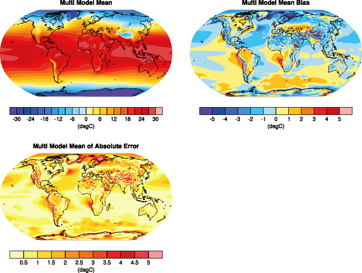
Fig. 150 Figure 9.2 a,b,c: Annual-mean surface air temperature for the period 1980-2005. a) multi-model mean, b) bias as the difference between the CMIP5 multi-model mean and the climatology from ERA-Interim (Dee et al., 2011), c) mean absolute model error with respect to the climatology from ERA-Interim.

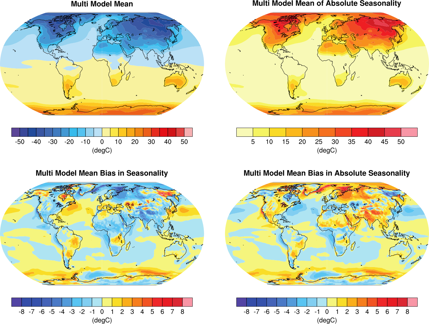
Fig. 151 Figure 9.3: Multi model values for seasonality of near-surface temperature, from top left to bottom right: mean, mean of absolute seasonality, mean bias in seasonality, mean bias in absolute seasonality. Reference dataset: ERA-Interim.

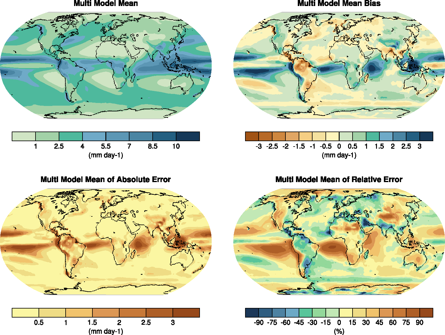
Fig. 152 Figure 9.4: Annual-mean precipitation rate (mm day-1) for the period 1980-2005. a) multi-model mean, b) bias as the difference between the CMIP5 multi-model mean and the climatology from the Global Precipitation Climatology Project (Adler et al., 2003), c) multi-model mean absolute error with respect to observations, and d) multi-model mean error relative to the multi-model mean precipitation itself.

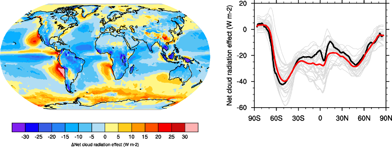
Fig. 153 Figure 9.5: Climatological (1985-2005) annual-mean cloud radiative effects in Wm-2 for the CMIP5 models against CERES EBAF (2001-2011) in Wm-2. Top row shows the shortwave effect; middle row the longwave effect, and bottom row the net effect. Multi-model-mean biases against CERES EBAF 2.6 are shown on the left, whereas the right panels show zonal averages from CERES EBAF 2.6 (black), the individual CMIP5 models (thin gray lines), and the multi-model mean (thick red line).

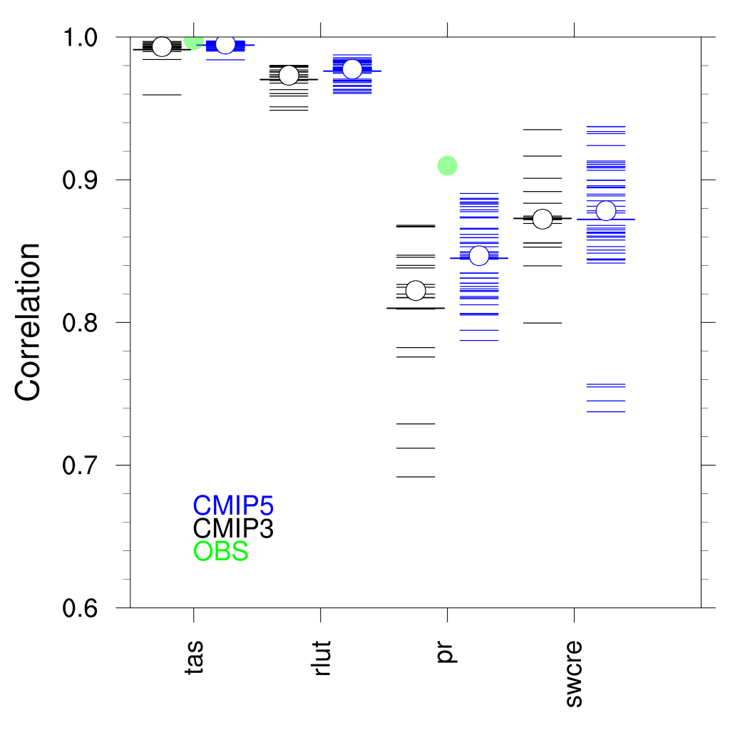
Fig. 154 Figure 9.6: Centered pattern correlations between models and observations for the annual mean climatology over the period 1980–1999. Results are shown for individual CMIP3 (black) and CMIP5 (blue) models as thin dashes, along with the corresponding ensemble average (thick dash) and median (open circle). The four variables shown are surface air temperature (TAS), top of the atmosphere (TOA) outgoing longwave radiation (RLUT), precipitation (PR) and TOA shortwave cloud radiative effect (SW CRE). The correlations between the reference and alternate observations are also shown (solid green circles).

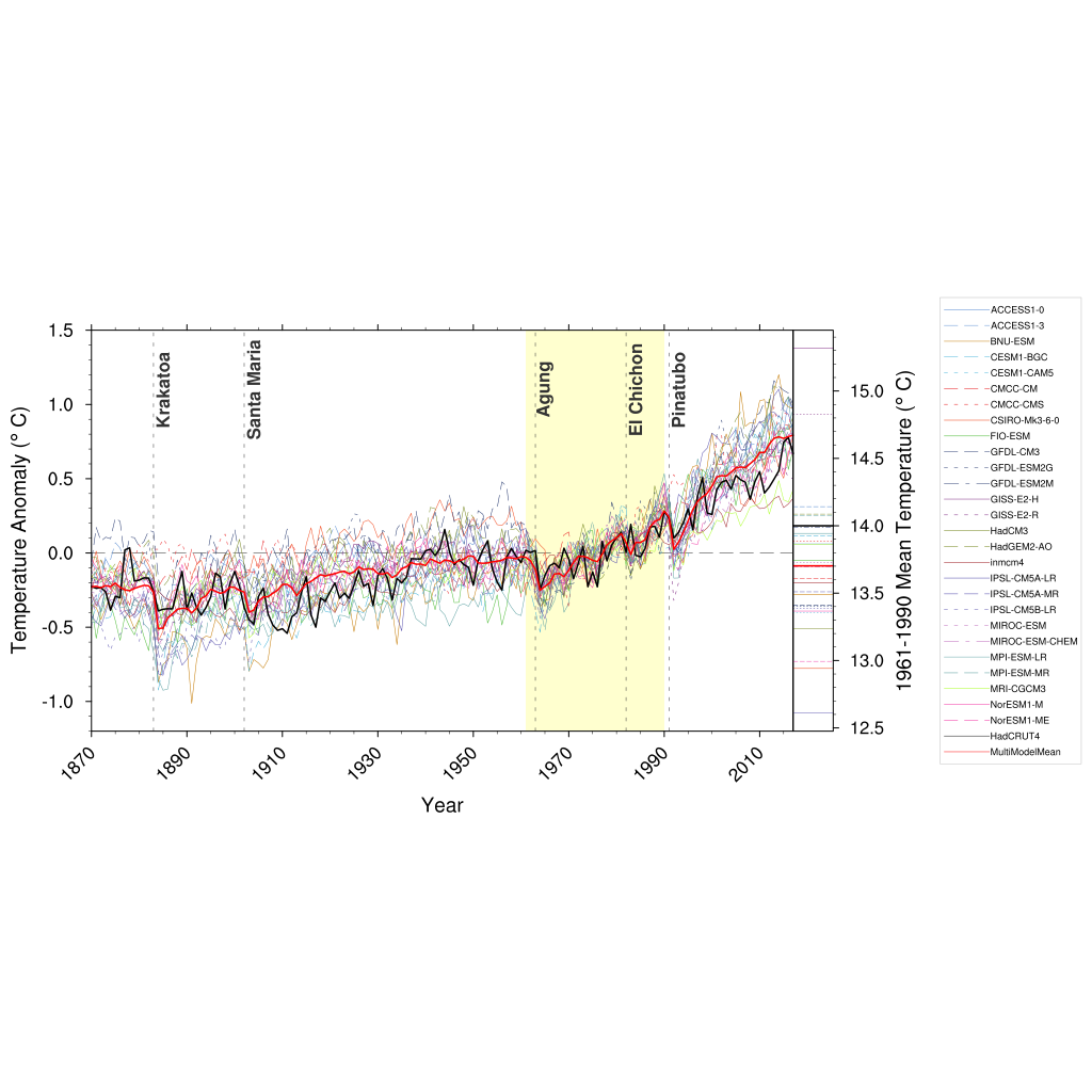
Fig. 155 Figure 9.8: Observed and simulated time series of the anomalies in annual and global mean surface temperature. All anomalies are differences from the 1961-1990 time-mean of each individual time series. The reference period 1961-1990 is indicated by yellow shading; vertical dashed grey lines represent times of major volcanic eruptions. Single simulations for CMIP5 models (thin lines); multi-model mean (thick red line); different observations (thick black lines). Dataset pre-processing like described in Jones et al., 2013.

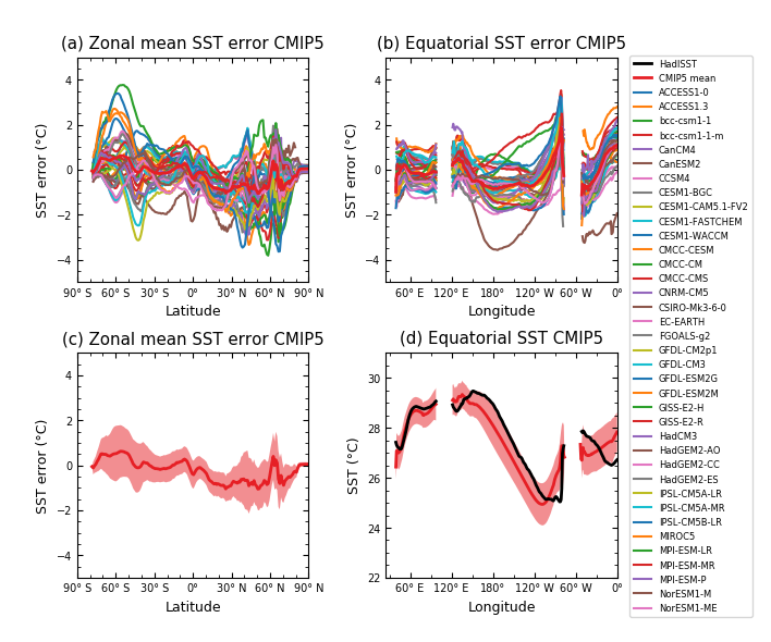
Fig. 156 Figure 9.14: (a) Zonally averaged sea surface temperature (SST) error in CMIP5 models. (b) Equatorial SST error in CMIP5 models. (c) Zonally averaged multi-model mean SST error for CMIP5 together with inter-model standard deviation (shading). (d) Equatorial multi-model mean SST in CMIP5 together with inter-model standard deviation (shading) and observations (black). Model climatologies are derived from the 1979-1999 mean of the historical simulations. The Hadley Centre Sea Ice and Sea Surface Temperature (HadISST) (Rayner et al., 2003) observational climatology for 1979-1999 is used as a reference for the error calculation (a), (b), and (c); and for observations in (d).

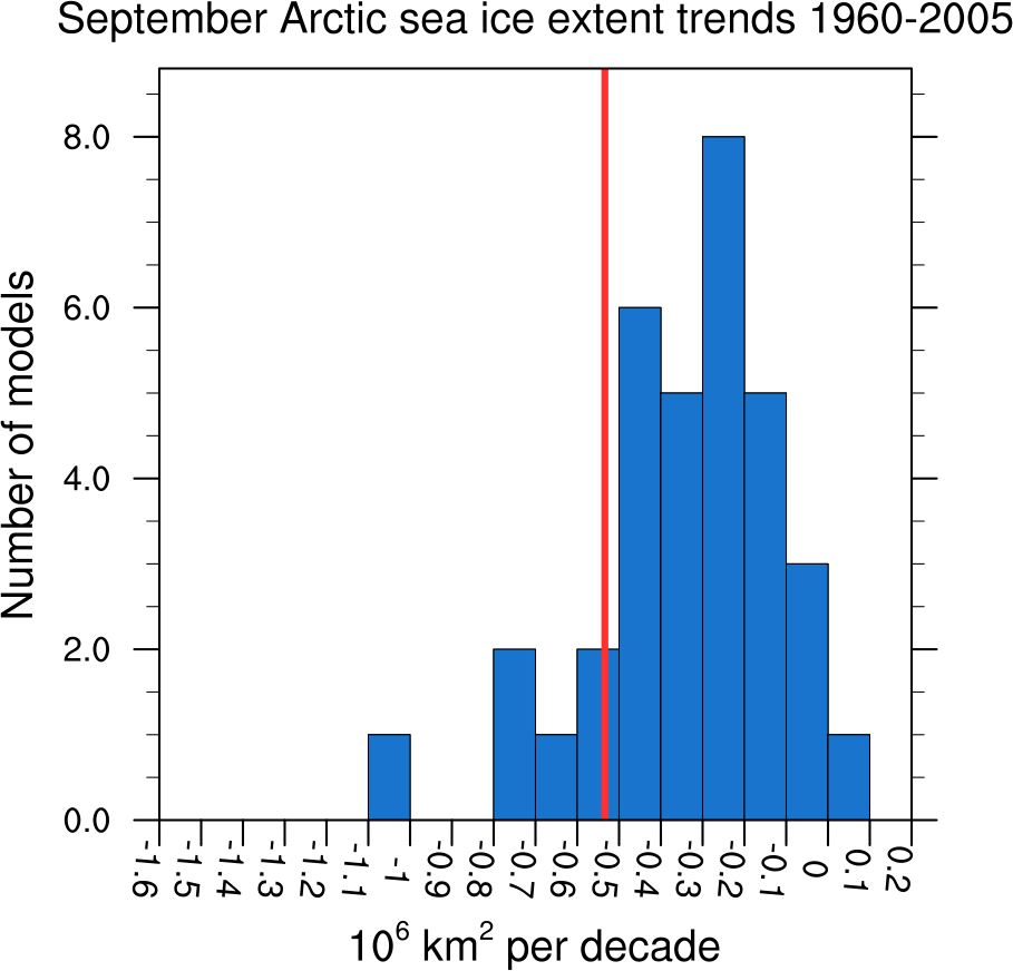
Fig. 157 Figure 9.24c: Sea ice extent trend distribution for the Arctic in September.

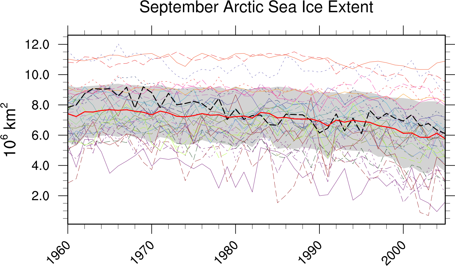
Fig. 158 Figure 9.24a: Time series of total sea ice area and extent (accumulated) for the Arctic in September including multi-model mean and standard deviation.

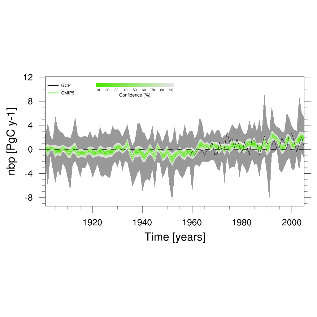
Fig. 159 Figure 9.26 (bottom): Ensemble-mean global land carbon uptake in the CMIP5 ESMs for the historical period 1900–2005. For comparison, the observation-based estimates provided by the Global Carbon Project (GCP) are also shown (black line). The confidence limits on the ensemble mean are derived by assuming that the CMIP5 models come from a t-distribution. The grey areas show the range of annual mean fluxes simulated across the model ensemble.

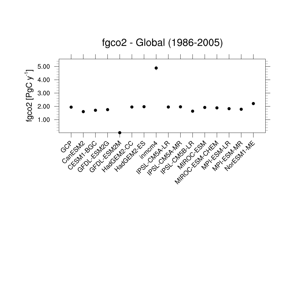
Fig. 160 Figure 9.27 (top): Simulation of global mean atmosphere–ocean CO2 fluxes (“fgCO2”) by ESMs for the period 1986–2005. For comparison, the observation-based estimates provided by Global Carbon Project (GCP) are also shown. The error bars for the ESMs and observations represent interannual variability in the fluxes, calculated as the standard deviation of the annual means over the period 1986–2005.

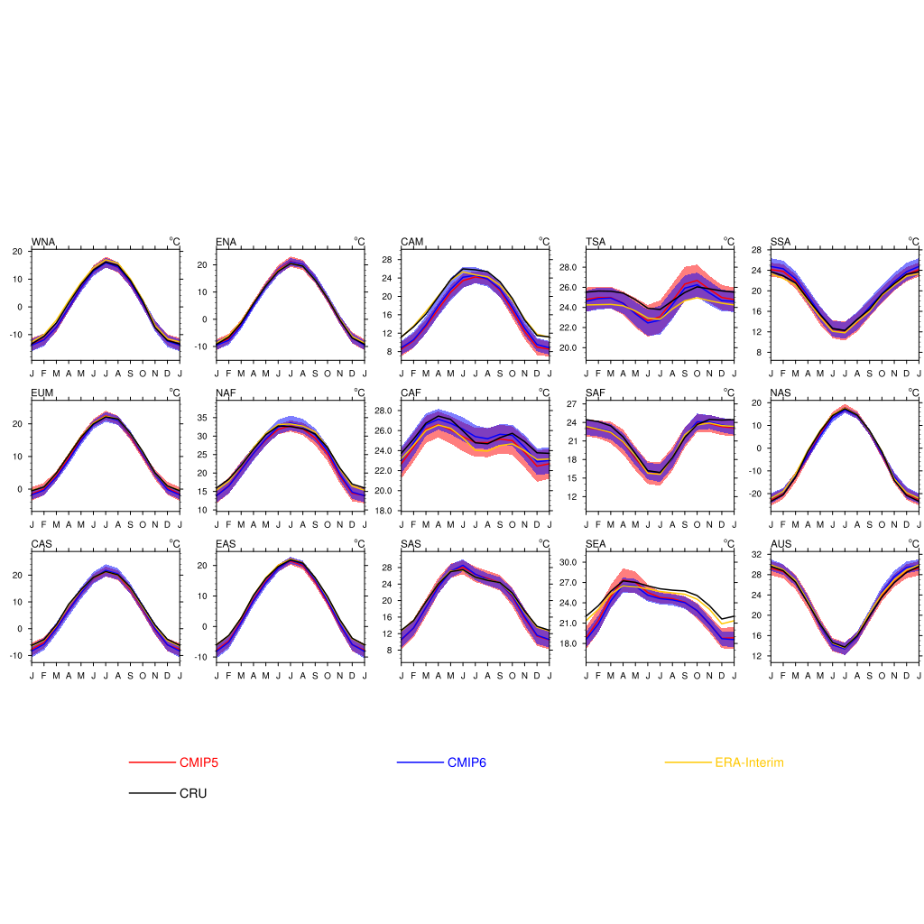
Fig. 161 Figure 9.38tas: Mean seasonal cycle for surface temperature (tas) as multi model mean of 38 CMIP5 and 22 CMIP6 models as well as CRU and ERA-Interim reanalysis data averaged for 1980-2005 over land in different regions: Western North America (WNA), Eastern North America (ENA), Central America (CAM), Tropical South America (TSA), Southern South America (SSA), Europe and Mediterranean (EUM), North Africa (NAF), Central Africa (CAF), South Africa (SAF), North Asia (NAS), Central Asia (CAS), East Asia (EAS), South Asia (SAS), Southeast Asia (SEA), and Australia (AUS). Similar to Fig. 9.38a from Flato et al. (2013), CMIP6 instead of CMIP3 and set of CMIP5 models used different.

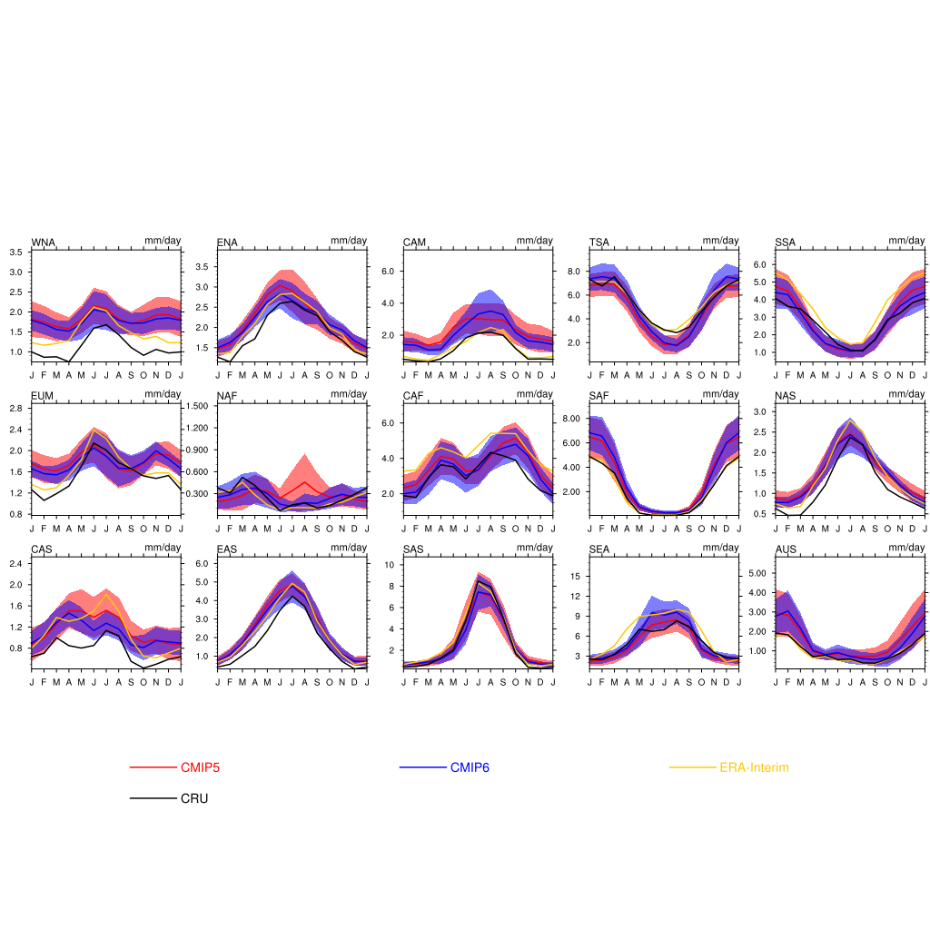
Fig. 162 Figure 9.38pr: Mean seasonal cycle for precipitation (pr) as multi model mean of 38 CMIP5 and 22 CMIP6 models as well as CRU and ERA-Interim reanalysis data averaged for 1980-1999 over land in different regions: Western North America (WNA), Eastern North America (ENA), Central America (CAM), Tropical South America (TSA), Southern South America (SSA), Europe and Mediterranean (EUM), North Africa (NAF), Central Africa (CAF), South Africa (SAF), North Asia (NAS), Central Asia (CAS), East Asia (EAS), South Asia (SAS), Southeast Asia (SEA), and Australia (AUS). Similar to Fig. 9.38b from Flato et al. (2013), CMIP6 instead of CMIP3 and set of CMIP5 models used different.

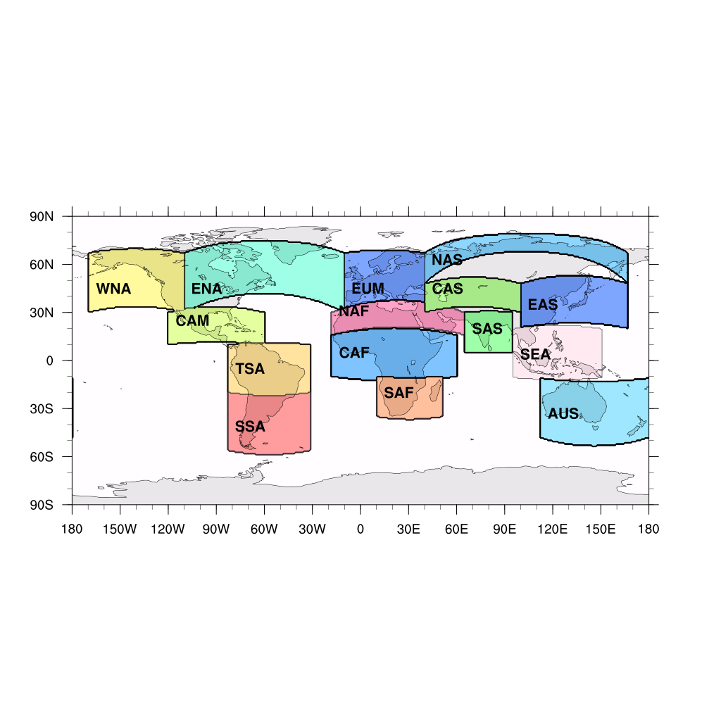
Fig. 163 Figure 9.38reg: Positions of the regions used in Figure 9.38.

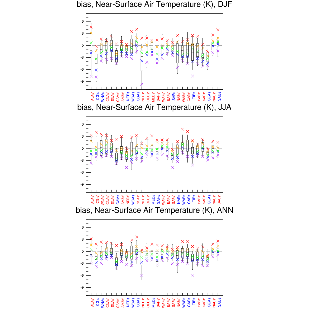
Fig. 164 Figure 9.39tas: Box and whisker plots showing the 5th, 25th, 50th, 75th and 95th percentiles of the seasonal- and annual mean biases for surface temperature (tas) for 1980-2005 between 38 CMIP5 models (box and whiskers) or 22 CMIP6 models (crosses) and CRU data. The regions are: Alaska/NW Canada (ALAs), Eastern Canada/Greenland/Iceland (CGIs), Western North America(WNAs), Central North America (CNAs), Eastern North America (ENAs), Central America/Mexico (CAMs), Amazon (AMZs), NE Brazil (NEBs), West Coast South America (WSAs), South-Eastern South America (SSAs), Northern Europe (NEUs), Central Europe (CEUs), Southern Europe/the Mediterranean (MEDs), Sahara (SAHs), Western Africa (WAFs), Eastern Africa (EAFs), Southern Africa (SAFs), Northern Asia (NASs), Western Asia (WASs), Central Asia (CASs), Tibetan Plateau (TIBs), Eastern Asia (EASs), Southern Asia (SASs), Southeast Asia (SEAs), Northern Australia (NASs) and Southern Australia/New Zealand (SAUs). The positions of these regions are defined following (Seneviratne et al., 2012) and differ from the ones in Fig. 9.38. Similar to Fig. 9.39 a,c,e from Flato et al. (2013), CMIP6 instead of CMIP3 and set of CMIP5 models used different.

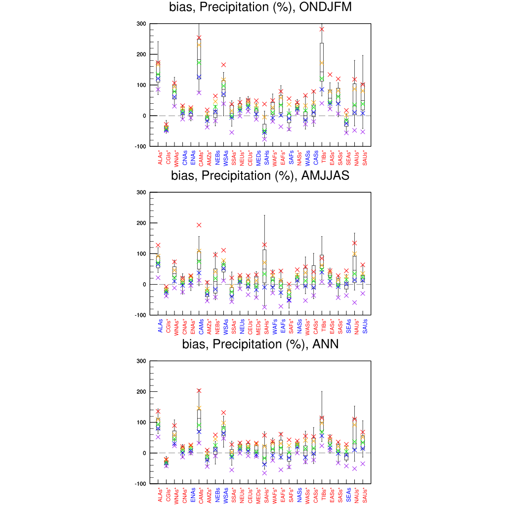
Fig. 165 Figure 9.39pr: Box and whisker plots showing the 5th, 25th, 50th, 75th and 95th percentiles of the seasonal- and annual mean biases for precipitation (pr) for 1980-2005 between 38 CMIP5 models (box and whiskers) or 22 CMIP6 models (crosses) and CRU data. The regions are: Alaska/NW Canada (ALAs), Eastern Canada/Greenland/Iceland (CGIs), Western North America(WNAs), Central North America (CNAs), Eastern North America (ENAs), Central America/Mexico (CAMs), Amazon (AMZs), NE Brazil (NEBs), West Coast South America (WSAs), South-Eastern South America (SSAs), Northern Europe (NEUs), Central Europe (CEUs), Southern Europe/the Mediterranean (MEDs), Sahara (SAHs), Western Africa (WAFs), Eastern Africa (EAFs), Southern Africa (SAFs), Northern Asia (NASs), Western Asia (WASs), Central Asia (CASs), Tibetan Plateau (TIBs), Eastern Asia (EASs), Southern Asia (SASs), Southeast Asia (SEAs), Northern Australia (NASs) and Southern Australia/New Zealand (SAUs). The positions of these regions are defined following (Seneviratne et al., 2012) and differ from the ones in Fig. 9.38. Similar to Fig. 9.39 b,d,f from Flato et al. (2013), CMIP6 instead of CMIP3 and set of CMIP5 models used different.

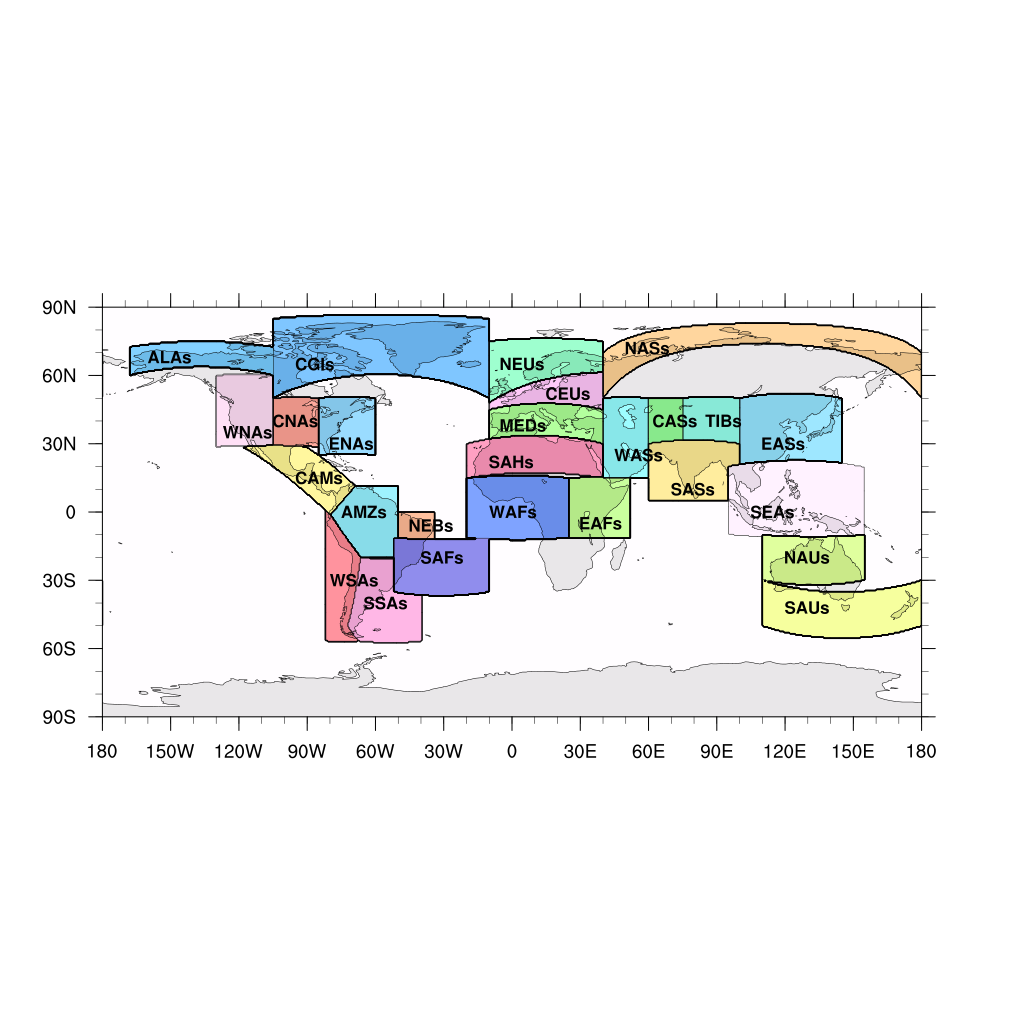
Fig. 166 Figure 9.39reg: Positions of the regions used in Figure 9.39.

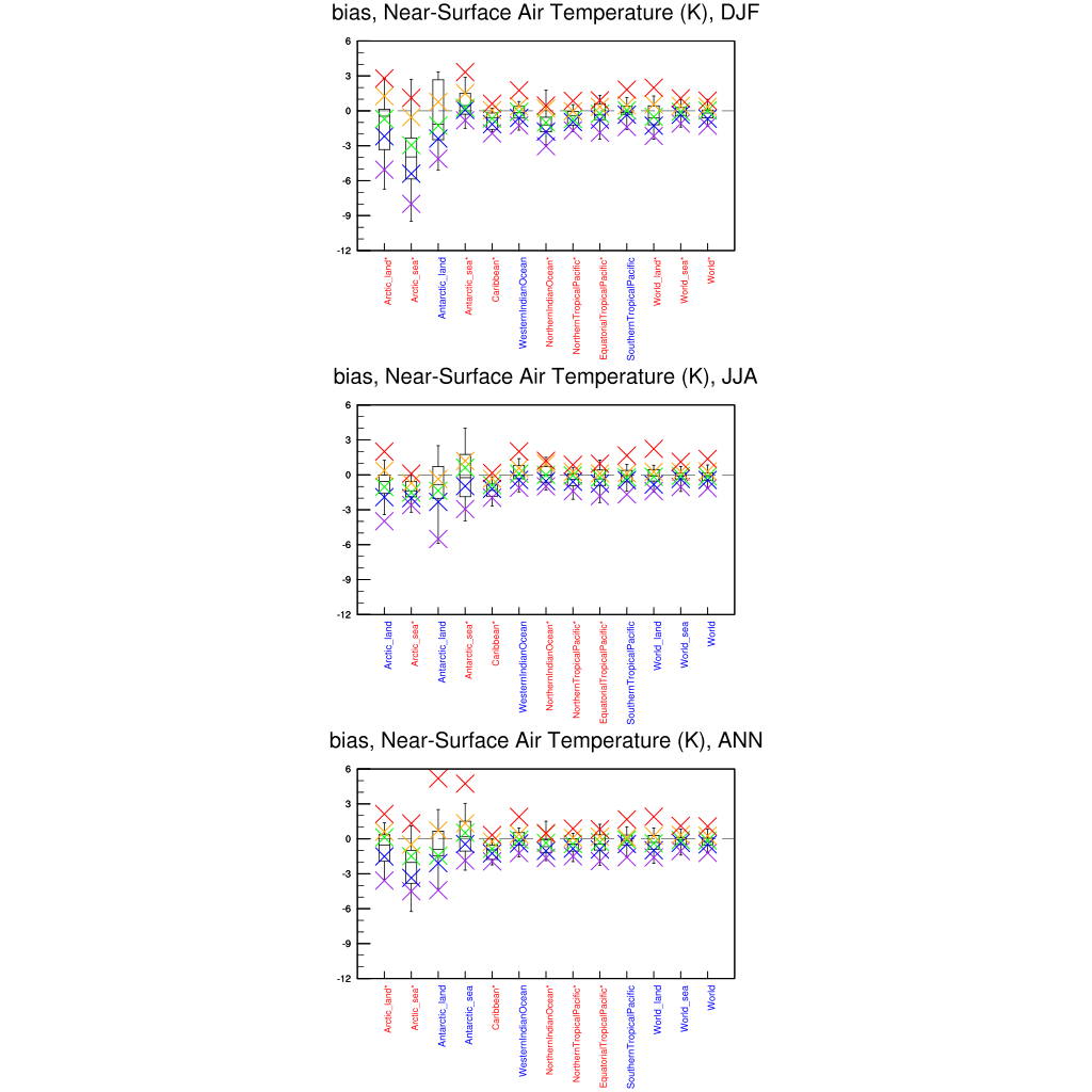
Fig. 167 Figure 9.40tas: Box and whisker plots showing the 5th, 25th, 50th, 75th and 95th percentiles of the seasonal- and annual mean biases for surface temperature (tas) for oceanic and polar regions between 38 CMIP5 (box and whiskers) or 22 CMIP6 (crosses) models and ERA-Interim data for 1980–2005.

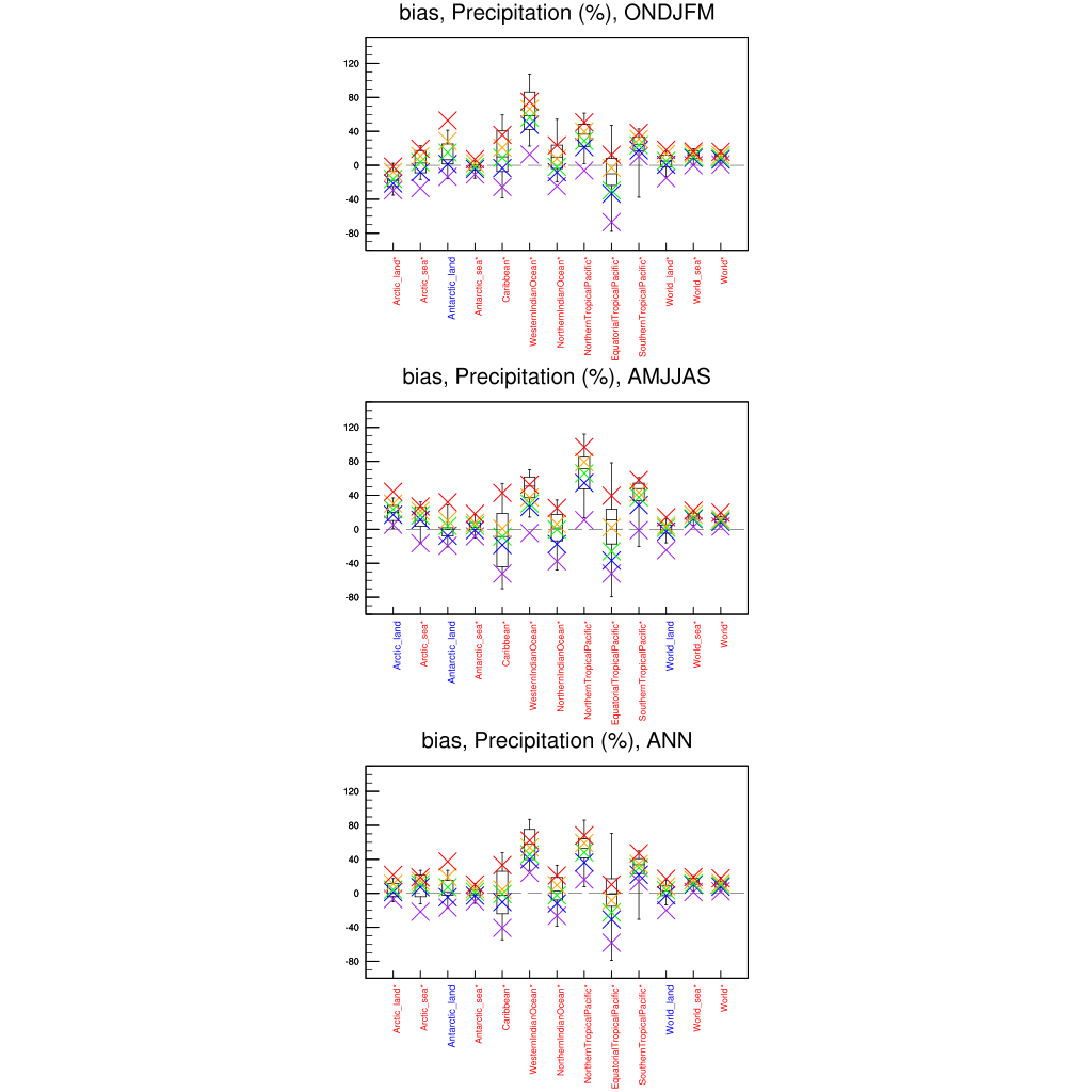
Fig. 168 Figure 9.40pr: Box and whisker plots showing the 5th, 25th, 50th, 75th and 95th percentiles of the seasonal- and annual mean biases for precipitation (pr) for oceanic and polar regions between 38 CMIP5 (box and whiskers) or 22 CMIP6 (crosses) models and Global Precipitation Climatology Project - Satellite-Gauge (GPCP-SG) data for 1980–2005.

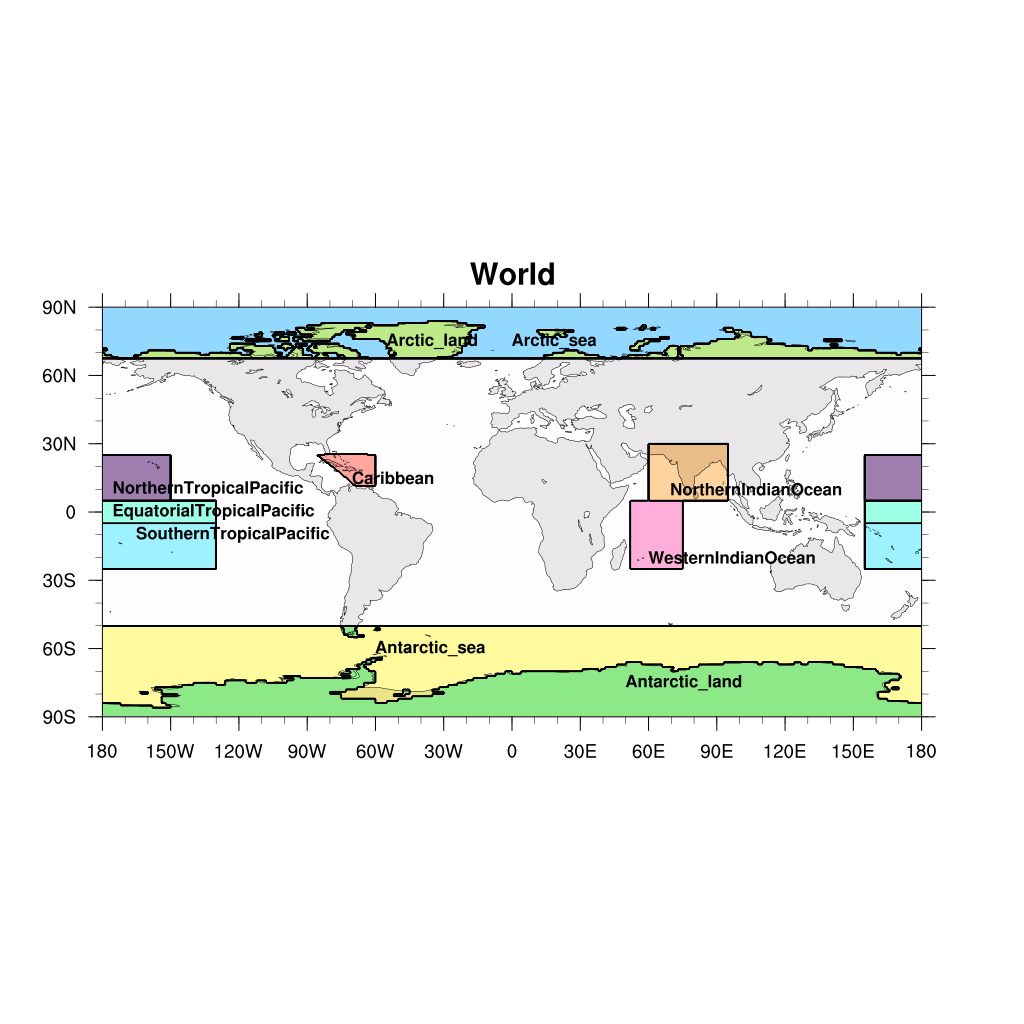
Fig. 169 Figure 9.40reg: Positions of the regions used in Figure 9.40.

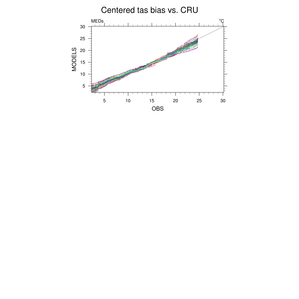
Fig. 170 Figure 9.41b: Ranked modelled versus ERA-Interim mean temperature for 38 CMIP5 models in the Mediterranean region for 1961–2000.

Fig. 171 Figure 9.42a: Equilibrium climate sensitivity (ECS) against the global mean surface air temperature of CMIP5 models, both for the period 1961-1990 (larger symbols) and for the pre-industrial control runs (smaller symbols).

Fig. 172 Figure 9.42b: Transient climate response (TCR) against equilibrium climate sensitivity (ECS) for CMIP5 models.

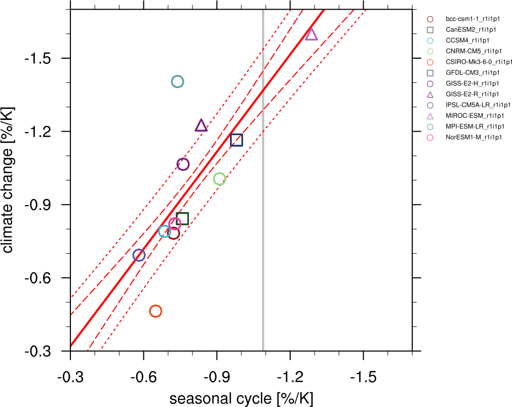
Fig. 173 Figure 9.45a: Scatterplot of springtime snow-albedo effect values in climate change vs. springtime \(\Delta \alpha_s\)/\(\Delta T_s\) values in the seasonal cycle in transient climate change experiments (CMIP5 historical experiments: 1901-2000, RCP4.5 experiments: 2101-2200).