Implied heat transport from Top of Atmosphere fluxes

Overview

This recipe calculates the implied horizontal heat transport (IHT) due to the spatial anomalies of radiative fluxes at the top of the atmosphere (TOA). The regional patterns of implied heat transport for different components of the TOA fluxes are calculated by solving the Poisson equation with the flux components as source terms. It reproduces the plots in Pearce and Bodas-Salcedo (2023) when the input data is CERES EBAF.

Available recipes and diagnostics

Recipes are stored in esmvaltool/recipes/

• recipe_iht_toa.yml calculates the IHT maps for the following radiative fluxes:

  • Total net, SW net, LW net (Figure 2).

  • Total CRE, SW CRE, LW CRE (Figure 4).

  • All-sky and clear-sky reflected SW (Figure 5).

  • The meridional heat transports (MHT) of the fluxes above (Figures 1 and 3).

Diagnostics are stored in esmvaltool/diag_scripts/iht_toa/

• single_model_diagnostics.py: driver script that produces the plots.

• poisson_solver.py: solver that calculates the IHTs.

User settings in recipe

There are no user settings in this recipe.

Variables

• rlut (atmos, monthly, longitude latitude time)

• rlutcs (atmos, monthly, longitude latitude time)

• rsutcs (atmos, monthly, longitude latitude time)

• rsut (atmos, monthly, longitude latitude time)

• rsdt (atmos, monthly, longitude latitude time)

Observations and reformat scripts

• CERES-EBAF

References

• Pearce, F. A., and A. Bodas-Salcedo, 2023: Implied Heat Transport from CERES Data: Direct Radiative Effect of Clouds on Regional Patterns and Hemispheric Symmetry. J. Climate, 36, 4019–4030, doi: 10.1175/JCLI-D-22-0149.1.

Example plots

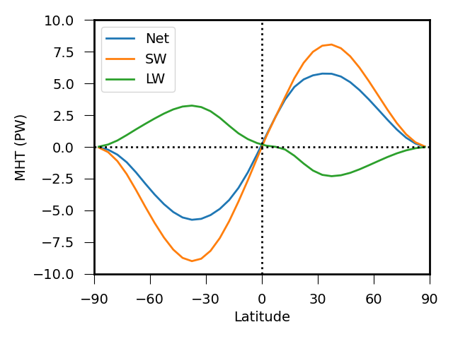
Fig. 42 The implied heat transport due to the total net flux (blue), split into the contributions from the SW (orange) and LW (green).

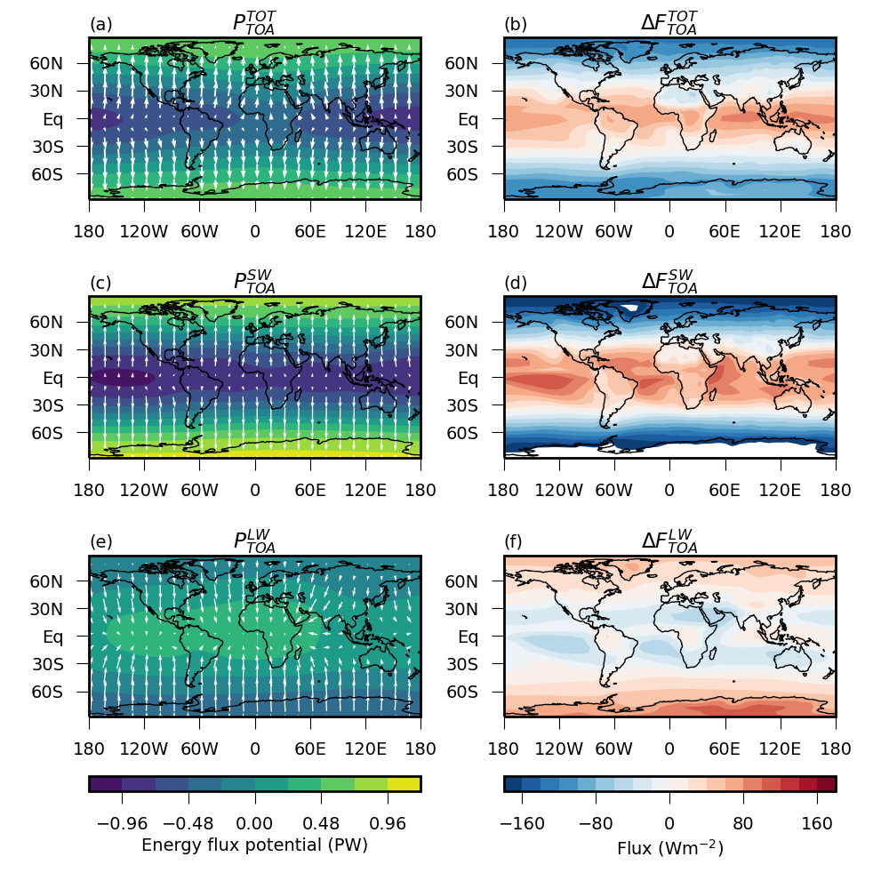
Fig. 43 The energy flux potentials for (a) TOT, (c) SW, and (e) LW fluxes, alongside maps of the spatial anomalies of the fluxes [(b),(d),(f) flux minus global average flux, respectively]. The implied heat transport is calculated as the gradient of the energy flux potential, shown by the white vector arrows for a subset of points to give the overall transport pattern. Heat is directed from the blue minima of the potential field to yellow maxima, with the magnitude implied by the density of contours. All maps of the same type share the same color bar at the bottom of the column.

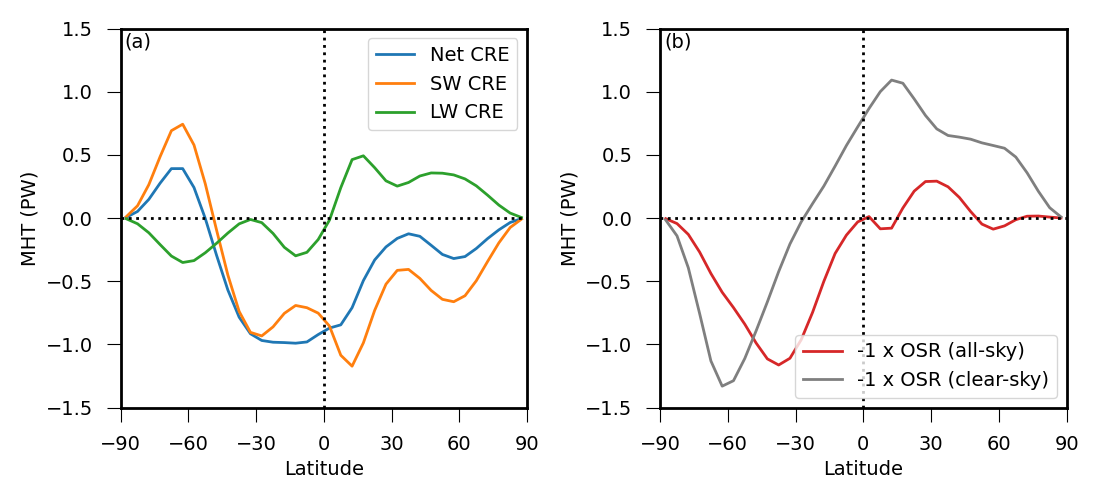
Fig. 44 Direct radiative effects of clouds on the meridional heat transport. (a) Contributions from TOT CRE (blue), SW CRE (orange), and LW CRE (green) fluxes. (b) Contributions from all-sky and clear-sky OSR. In (b), both curves have been multiplied by −1 such that positive heat transport is northward.

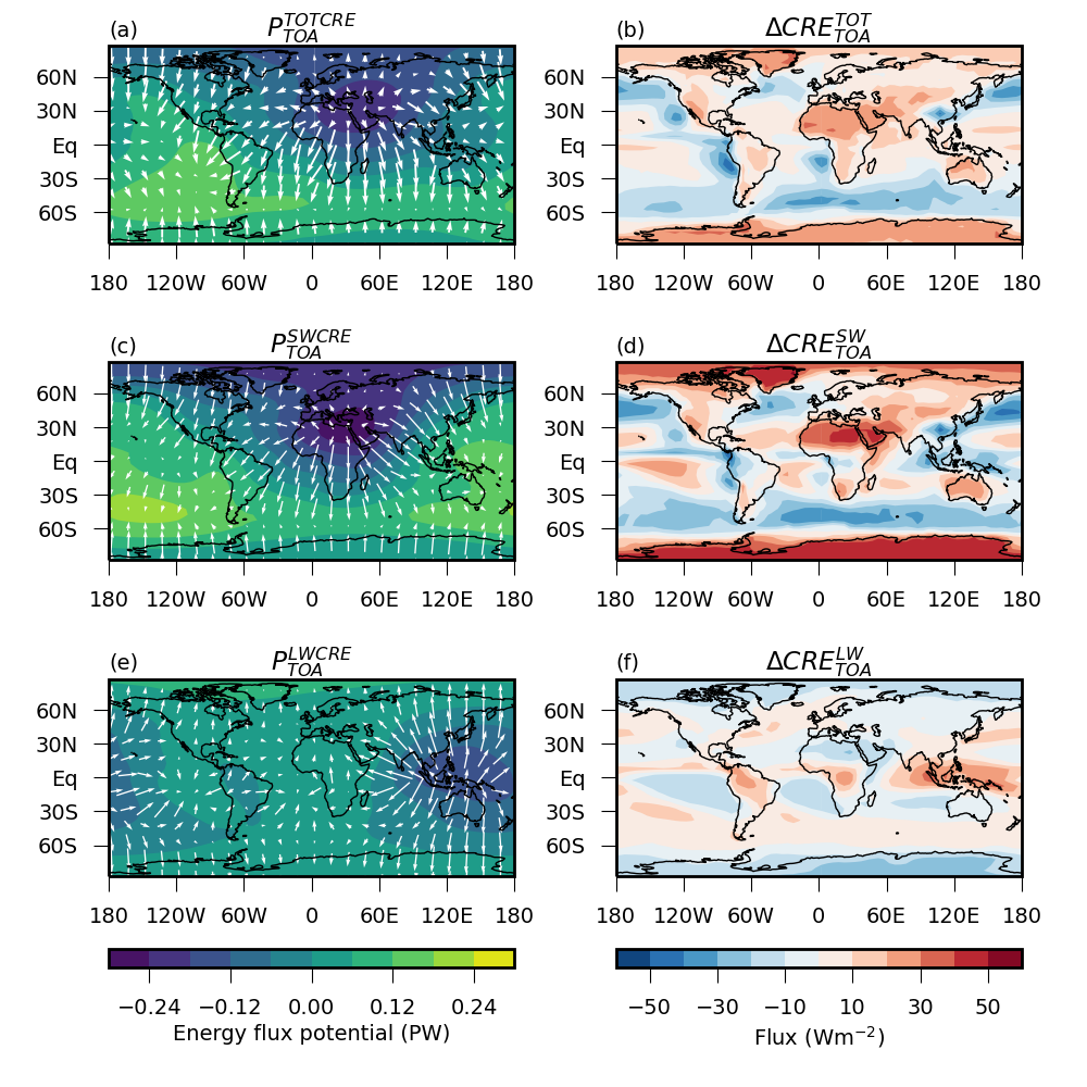
Fig. 45 As in Fig. 43, but for the implied heat transport associated with (a),(b) TOT CRE, (c),(d) SW CRE, and (e),(f) LW CRE fluxes.

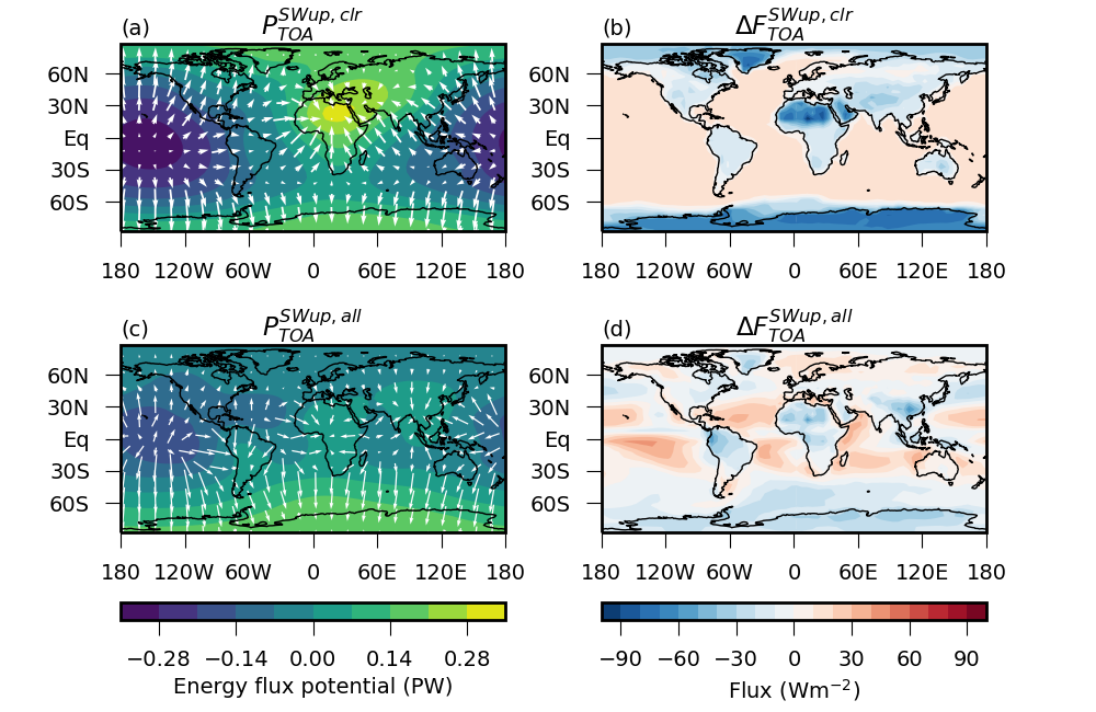
Fig. 46 As in Fig. 43, but for (a), (b) clear-sky and (c), (d) all-sky reflected SW flux.

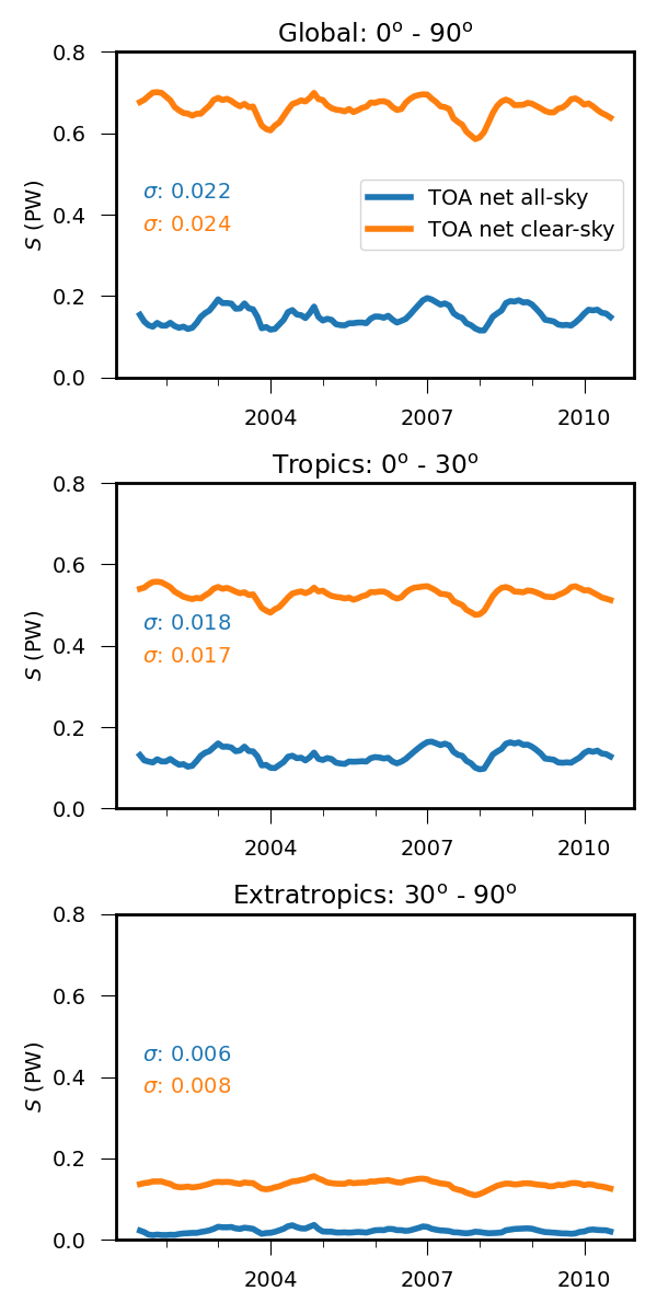
Fig. 47 A measure of the symmetry between heat transport in the Northern and Southern Hemispheres, calculated for the 12-month running mean of TOT MHT in the regions: (a) the full hemisphere, (b) from the equator to 30°, and (c) 30° to 90°. Symmetry values obtained when including (blue) and excluding (orange) the effect of clouds. The climatological symmetry values for the two cases are shown as the black lines in each subplot, dashed and dotted, respectively. The standard deviations of the time series are shown in each plot.