Climate model projections from the ScenarioMIP of CMIP6#
Overview#
This recipe is implemented into ESMValTool to evaluate the temperature and precipitation changes from the ScenarioMIP of CMIP6. It produces the original plots and tables of Tebaldi et al. (2021), https://doi.org/10.5194/esd-12-253-2021
Available recipe and diagnostics#
Recipe is stored in esmvaltool/recipes/
recipe_tebaldi21esd.yml
Diagnostics are stored in esmvaltool/diag_scripts/tebaldi21esd/
calc_timeseries_across_realization_stddev_runave.ncl: computes time series of ensemble spreads (i.e., inter-member standard deviations). One dataset is used for resampling subsets of 10 members.
calc_cmip6_and_cmip5_pattern_diff_scaleT.ncl: computes the pattern difference between the CMIP6 multi-model mean change and the CMIP5 multi-model mean change.
calc_IAV_hatching.ncl: computes the interannual variability (IAV) over piControl runs, either over the whole time period or in chunks over some years.
calc_pattern_diff_scaleT.ncl: computes the map of multi-model mean change scaled by global T change.
calc_pattern_stippling_hatching.ncl: computes the map of multi-model mean change with stippling for significant region and hatching for non-significant region. Significant is where the multi-model mean change is greater than two standard deviations of the internal variability and where at least 90% of the models agree on the sign of change. Not significant is where the multi-model mean change is less than one standard deviation of internal variability.
calc_pattern_intermodel_stddev_scaleT.ncl: computes the intermodel standard deviation of the change scaled by global T change standard deviation of the change scaled by global T change
calc_pattern_interscenario_stddev_scaleT.ncl: computes the interscenario standard deviation of the change scaled by global T change
calc_pattern_stddev_scaleT.ncl: computes the standard deviation of the change scaled by global T change
calc_pattern_comparison.ncl: computes the difference between the patterns of multi-model mean change of two different scenarios (ex: SSP4-6.0 and SSP4-3.4)
calc_table_changes.ncl: computes the changes (mean and spreads) for the specified scenarios and time periods relative to the historical baseline.
calc_table_warming_level.ncl: computes the warming level crossing year (mean, five percent and ninety-five percent quantiles of crossing years) for specified scenarios and warming levels.
calc_timeseries_mean_spread_runave.ncl: computes multi-model time series of change against historical baseline for specified scenarios with spread. A running average with specified window is performed.
calc_timeseries_mean_spread_ssp4.ncl: computes multi-model time series of change against historical baseline for specified ssp434 and ssp460 with spread. A running average with specified window is performed.
calc_timeseries_mean_spread_ssp5.ncl: computes multi-model time series of change against historical baseline for ssp534-over and ssp585 with spread. A running average with specified window is performed.
plot_pattern.ncl: plots a pattern.
plot_table_changes: plots a table of the multi-model mean and spread for specified scenarios and periods.
plot_table_warming_level.ncl: plots a table of warming level crossing years for specified scenarios (columns) and warming levels (rows).
plot_timeseries_mean_spread_3scenarios.ncl: plots time series (multi- model mean and spread) for 3 scenarios.
plot_timeseries_mean_spread_constrained_projections.ncl: plot time series with brackets for constrained projections.
plot_timeseries_mean_spread.ncl: plot time series (multi-model mean and spread) for 5 scenarios.
plot_timeseries_mean_spread_rightaxis_5scen.ncl: plot time series (multi-model mean and spread) for 5 scenarios and with an additional right axis.
plot_timeseries_mean_spread_ssp4.ncl: plot time series for two ssp4 scenarios.
plot_timeseries_mean_spread_ssp5.ncl: plot time series for two ssp5 scenarios.
plot_timeseries_across_realization_stddev_runave.ncl: plot time series of inter-member standard deviation.
User settings in recipe#
Script calc_timeseries_across_realization_stddev_runave.ncl
Required settings for script
scenarios: list with scenarios included in figure
syears: list with start years in time periods (e.g. start of historical period and SSPs)
eyears: list with end years in time periods (end year of historical runs and SSPs)
begin_ref_year: start year of reference period (e.g. 1995)
end_ref_year: end year of reference period (e.g. 2014)
n_samples: number of samples of size 10 to draw among all the ensembles of sampled_model
sampled_model: name of dataset on which to sample
runave_window: size window used for the centered running average
Script calc_cmip6_and_cmip5_pattern_diff_scaleT.ncl
Required settings for script
scenarios_cmip5: list of CMIP5 scenarios included in figure
scenarios_cmip6: list of CMIP6 scenarios included in figure
periods: list with start years of periods to be included
time_avg: time_avg: time averaging (“annualclim”, “seasonalclim”)
Optional settings for script
percent: determines if difference expressed in percent (0, 1, default= 0)
Script calc_IAV_hatching.ncl
Required settings for script
time_avg: time_avg: time averaging (“annualclim”, “seasonalclim”) needs to be consistent with calc_pattern_stippling_hatching.ncl
Optional settings for script
periodlength: length of period in years to calculate variability over, default is total time period
iavmode: calculate IAV from multi-model mean or save individual models (“each”: save individual models, “mmm”: multi-model mean, default), needs to be consistent with calc_pattern_stippling_hatching.ncl
Script calc_pattern_diff_scaleT.ncl
Required settings for script
scenarios: list with scenarios included in figure
periods: list with start years of periods to be included
time_avg: time_avg: time averaging (“annualclim”, “seasonalclim”)
Script calc_pattern_stippling_hatching.ncl
Required settings for script
ancestors: variable and diagnostics that calculated interannual variability for stiplling and hatching
time_avg: time_avg: time averaging (“annualclim”, “seasonalclim”) needs to be consistent with calc_IAV_hatching.ncl
scenarios: list with scenarios to be included
periods: list with start years of periods to be included
labels: list with labels to use in legend depending on scenarios
sig: plot stippling for significance? (True, False)
not_sig: plot hatching for uncertainty? (True, False)
Optional settings for script
seasons: list with season index if time_avg is “seasonalclim” (then seasons is required), DJF:0, MAM:1, JJA:2, SON:3
iavmode: calculate IAV from multi-model mean or save individual models (“each”: save individual models, “mmm”: multi-model mean, default), needs to be consistent with calc_IAV_hatching.ncl
percent: determines if difference expressed in percent (0, 1, default = 0)
Script calc_pattern_intermodel_stddev_scaleT.ncl
Required settings for script
scenarios: list with scenarios included in figure
periods: list with start years of periods to be included
time_avg: time_avg: time averaging (“annualclim”, “seasonalclim”)
Script calc_pattern_interscenario_stddev_scaleT.ncl
Required settings for script
scenarios: list with scenarios included in figure
periods: list with start years of periods to be included
time_avg: time_avg: time averaging (“annualclim”, “seasonalclim”)
Script calc_pattern_stddev_scaleT.ncl
Required settings for script
scenarios: list with scenarios included in figure
periods: list with start years of periods to be included
time_avg: time_avg: time averaging (“annualclim”, “seasonalclim”)
Script calc_pattern_comparison.ncl
Required settings for script
scenarios: list with two scenarios included in figure. The last scenario is taken as reference. For example to compute the difference of pattern between SSP4-6.0 and SSP4-3.4, the scenario ssp460 should be the last element of the list.
periods: list with start years of periods to be included
time_avg: time_avg: time averaging (“annualclim”, “seasonalclim”)
label: label of periods
Script calc_table_changes.ncl
Required settings for script
scenarios: list with scenarios included in the table
syears: list with start years of time periods to include in the table
eyears: list with end years of the time periods to include in the table
begin_ref_year: start year of historical baseline period (e.g. 1995)
end_ref_year: end year of historical baseline period (e.g. 2014)
spread: multiplier of standard deviation to calculate spread with (e.g. 1.64)
label: list of scenario names included in the table
Script calc_table_warming_level.ncl
Required settings for script
scenarios: list with scenarios included in the table
warming_levels: list of warming levels to include in the table
syears: list with start years of time periods (historical then SSPs)
eyears: list with end years of the time periods (historical then SSPs)
begin_ref_year: start year of historical baseline period (e.g. 1995)
end_ref_year: end year of historical baseline period (e.g. 2014)
offset: offset between current historical baseline and 1850-1900 period
label: list of scenario names included in the table
Script calc_timeseries_mean_spread_runave.ncl
Required settings for script
scenarios: list of scenarios to include
syears: list with start years of time periods (historical then SSPs)
eyears: list with end years of the time periods (historical then SSPs)
begin_ref_year: start year of historical baseline period (e.g. 1986)
end_ref_year: end year of historical baseline period (e.g. 2005)
Optional settings for script
runave_window: size of the window used to perform running average (default 11)
spread: how many standard deviations to calculate the spread with (default 1)
label: list of scenario names included in the legend
percent: determines if difference expressed in percent (0, 1, default = 0)
model_nr: whether to save number of models used for each scenario
Script calc_timeseries_mean_spread_ssp4.ncl
Required settings for script
scenarios: list of scenarios to include: ssp434 and ssp460
syears: list with start years of time periods (historical then SSPs)
eyears: list with end years of the time periods (historical then SSPs)
begin_ref_year: start year of historical baseline period (e.g. 1986)
end_ref_year: end year of historical baseline period (e.g. 2005)
Optional settings for script
runave_window: size of the window used to perform running average (default 11)
spread: how many standard deviations to calculate the spread with (default 1)
label: list of scenario names included in the legend
percent: determines if difference expressed in percent (0, 1, default = 0)
model_nr: whether to save number of models used for each scenario
Script calc_timeseries_mean_spread_ssp5.ncl
Required settings for script
scenarios: list of scenarios to include: ssp534-over, ssp585
syears: list with start years of time periods (historical then SSPs)
eyears: list with end years of the time periods (historical then SSPs)
begin_ref_year: start year of historical baseline period (e.g. 1986)
end_ref_year: end year of historical baseline period (e.g. 2005)
Optional settings for script
runave_window: size of the window used to perform running average (default 11)
spread: how many standard deviations to calculate the spread with (default 1)
label: list of scenario names included in the legend
percent: determines if difference expressed in percent (0, 1, default = 0)
model_nr: whether to save number of models used for each scenario
Script plot_pattern.ncl
Required settings for script
scenarios: list of scenarios
periods: list with start years of periods
ancestors: variable and diagnostics that calculated field to be plotted
Optional settings for script
projection: map projection, any valid ncl projection, default = Robinson
diff_levs: list with explicit levels for all contour plots
max_vert: maximum number of plots in vertical
max_hori: maximum number of plots in horizontal
model_nr: save number of model runs per period and scenario in netcdf to print in plot? (True, False, default = False)
colormap: alternative colormap, path to rgb file or ncl name
span: span whole colormap? (True, False, default = True)
pltname: alternative name for output plot, default is diagnostic + varname + time_avg
units: units written next to colorbar, e.g. (~F35~J~F~C)
sig: plot stippling for significance? (True, False)
not_sig: plot hatching for uncertainty? (True, False)
label: label to add in the legend
Script plot_table_changes.ncl
Required settings for script
ancestors: variable and diagnostics that calculated field to be plotted
scenarios: list of scenarios included in the figure
syears: list of start years of periods of interest
eyears: list of end years of periods of interest
label: list of labels of the scenarios
Optional settings for script
title: title of the plot
Script plot_table_warming_level.ncl
Required settings for script
scenarios: list of scenarios included in the figure
warming_levels: list of warming levels
syears: list of start years of historical and SSPs scenarios
eyears: list of end years of historical and SSPs scenarios
begin_ref_year: start year of reference period
end_ref_year: end year of reference period
label: list of labels of the scenarios
offset: offset between reference baseline and 1850-1900
Script plot_timeseries_mean_spread_3scenarios.ncl
Required settings for script
ancestors: variable and diagnostics that calculated field to be plotted
scenarios: list of scenarios included in the figure
syears: list of start years of historical and SSPs scenarios
eyears: list of end years of historical and SSPs scenarios
begin_ref_year: start year of reference period
end_ref_year: end year of reference period
label: list of labels of the scenarios
Optional settings for script
title: specify plot title
yaxis: specify y-axis title
ymin: minimim value on y-axis, default calculated from data
ymax: maximum value on y-axis
colormap: alternative colormap, path to rgb file or ncl name
model_nr: save number of model runs per period and scenario
styleset: color style
spread: how many standard deviations to calculate the spread with, default is 1, ipcc tas is 1.64
Script plot_timeseries_mean_spread_constrained_projections.ncl
Required settings for script
ancestors: variable and diagnostics that calculated field to be plotted
scenarios: list of scenarios included in the figure
syears: list of start years of historical and SSPs scenarios
eyears: list of end years of historical and SSPs scenarios
begin_ref_year: start year of reference period
end_ref_year: end year of reference period
label: list of labels of the scenarios
baseline_offset: offset between reference period (baseline) and 1850-1900
lower_constrained_projections: list of lower bounds of the constrained projections for the scenarios included in the same order as the scenarios
upper_constrained_projections: list of upper bounds of the constrained projections for the scenarios included in the same order as the scenarios
mean_constrained_projections: list of means of the constrained projections for the scenarios included in the same order as the scenarios
Optional settings for script
title: specify plot title
yaxis: specify y-axis title
ymin: minimim value on y-axis, default calculated from data
ymax: maximum value on y-axis
colormap: alternative colormap, path to rgb file or ncl name
model_nr: save number of model runs per period and scenario
styleset: color style
spread: how many standard deviations to calculate the spread with, default is 1, ipcc tas is 1.64
Script plot_timeseries_mean_spread.ncl
Required settings for script
ancestors: variable and diagnostics that calculated field to be plotted
scenarios: list of scenarios included in the figure
syears: list of start years of historical and SSPs scenarios
eyears: list of end years of historical and SSPs scenarios
begin_ref_year: start year of reference period
end_ref_year: end year of reference period
label: list of labels of the scenarios
Optional settings for script
title: specify plot title
yaxis: specify y-axis title
ymin: minimim value on y-axis, default calculated from data
ymax: maximum value on y-axis
colormap: alternative colormap, path to rgb file or ncl name
model_nr: save number of model runs per period and scenario
styleset: color style
spread: how many standard deviations to calculate the spread with, default is 1, ipcc tas is 1.64
Script plot_timeseries_mean_spread_rightaxis_5scen.ncl
Required settings for script
ancestors: variable and diagnostics that calculated field to be plotted
scenarios: list of scenarios included in the figure
syears: list of start years of historical and SSPs scenarios
eyears: list of end years of historical and SSPs scenarios
begin_ref_year: start year of reference period
end_ref_year: end year of reference period
rightaxis_offset: offset of the right axis relative to the left axis
label: list of labels of the scenarios
Optional settings for script
title: specify plot title
yaxis: specify y-axis title
ymin: minimim value on y-axis, default calculated from data
ymax: maximum value on y-axis
colormap: alternative colormap, path to rgb file or ncl name
model_nr: save number of model runs per period and scenario
styleset: color style
spread: how many standard deviations to calculate the spread with, default is 1, ipcc tas is 1.64
Script plot_timeseries_mean_spread_ssp4.ncl
Required settings for script
ancestors: variable and diagnostics that calculated field to be plotted
scenarios: list of scenarios included in the figure
syears: list of start years of historical and SSPs scenarios
eyears: list of end years of historical and SSPs scenarios
begin_ref_year: start year of reference period
end_ref_year: end year of reference period
label: list of labels of the scenarios
Optional settings for script
title: specify plot title
yaxis: specify y-axis title
ymin: minimim value on y-axis, default calculated from data
ymax: maximum value on y-axis
colormap: alternative colormap, path to rgb file or ncl name
model_nr: save number of model runs per period and scenario
styleset: color style
spread: how many standard deviations to calculate the spread with, default is 1, ipcc tas is 1.64
Script plot_timeseries_mean_spread_ssp5.ncl
Required settings for script
ancestors: variable and diagnostics that calculated field to be plotted
scenarios: list of scenarios included in the figure
syears: list of start years of historical and SSPs scenarios
eyears: list of end years of historical and SSPs scenarios
begin_ref_year: start year of reference period
end_ref_year: end year of reference period
label: list of labels of the scenarios
Optional settings for script
title: specify plot title
yaxis: specify y-axis title
ymin: minimim value on y-axis, default calculated from data
ymax: maximum value on y-axis
colormap: alternative colormap, path to rgb file or ncl name
model_nr: save number of model runs per period and scenario
styleset: color style
spread: how many standard deviations to calculate the spread with, default is 1, ipcc tas is 1.64
Script plot_timeseries_across_realization_stddev_runave.ncl
Required settings for script
ancestors: variable and diagnostics that calculated field to be plotted
scenarios: list of scenarios included in the figure
syears: list of start years of historical and SSPs scenarios
eyears: list of end years of historical and SSPs scenarios
begin_ref_year: start year of reference period
end_ref_year: end year of reference period
label: list of labels of the scenarios
n_samples: number of samples of size 10 to draw among all the ensembles of sampled_model only
sampled_model: name of dataset on which to sample
Optional settings for script
trend: whether the trend is calculated and displayed
runave_window: only used if trend is true, size window used for the centered running average
title: specify plot title
yaxis: specify y-axis title
ymin: minimim value on y-axis, default calculated from data
ymax: maximum value on y-axis
colormap: alternative colormap, path to rgb file or ncl name
Variables#
Note: These are the variables tested and used in the original paper.
tas (atmos, monthly mean, longitude latitude time)
pr (atmos, monthly mean, longitude latitude time)
However, the code is flexible and in theory other variables of the same kind can be used.
References#
Tebaldi, C., Debeire, K., Eyring, V., Fischer, E., Fyfe, J., Friedlingstein, P., Knutti, R., Lowe, J., O’Neill, B., Sanderson, B., van Vuuren, D., Riahi, K., Meinshausen, M., Nicholls, Z., Hurtt, G., Kriegler, E., Lamarque, J.-F., Meehl, G., Moss, R., Bauer, S. E., Boucher, O., Brovkin, V., Golaz, J.-C., Gualdi, S., Guo, H., John, J. G., Kharin, S., Koshiro, T., Ma, L., Olivié, D., Panickal, S., Qiao, F., Rosenbloom, N., Schupfner, M., Seferian, R., Song, Z., Steger, C., Sellar, A., Swart, N., Tachiiri, K., Tatebe, H., Voldoire, A., Volodin, E., Wyser, K., Xin, X., Xinyao, R., Yang, S., Yu, Y., and Ziehn, T.: Climate model projections from the Scenario Model Intercomparison Project (ScenarioMIP) of CMIP6, Earth Syst. Dynam., 12, 253-293, https://doi.org/10.5194/esd-12-253-2021
Example plots#
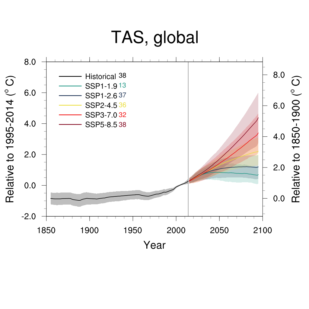
Fig. 263 Global average temperature time series (11-year running averages) of changes from current baseline (1995–2014, left axis) and pre-industrial baseline (1850–1900, right axis, obtained by adding a 0.84 ◦C offset) for SSP1-1.9, SSP1-2.6, SSP2-4.5, SSP3-7.0 and SSP5-8.5.#

Fig. 264 Patterns of temperature (a) and percent precipitation change (b) normalized by global average temperature change (averaged across CMIP6 models and all Tier 1 plus SSP1-1.9 scenarios).#
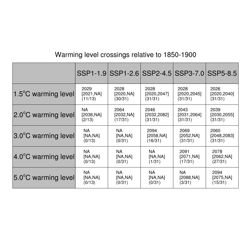
Fig. 265 Times (best estimate and range – in square brackets – based on the 5 %–95 % range of the ensemble after smoothing the trajectories by 11-year running means) at which various warming levels (defined as relative to 1850–1900) are reached according to simulations following, from left to right, SSP1-1.9, SSP1-2.6, SSP2-4.5, SSP3-7.0 and SSP5-8.5. Crossing of these levels is defined by using anomalies with respect to 1995–2014 for the model ensembles and adding the offset of 0.84 to derive warming from pre-industrial values. We use a common subset of 31 models for the Tier 1 scenarios and all available models (13) for SSP1-1.9, while Table A7 shows the result of using all available models under each scenario. The number of models available under each scenario and the number of models reaching a given warming level are shown in parentheses. However, the estimates are based on the ensemble means and ranges computed from all the models considered (13 or 31 in this case), not just from the models that reach a given level. An estimate marked as “NA” is to be interpreted as “not reaching that warming level by 2100”. In cases where the ensemble average remains below the warming level for the whole century, it is possible for the central estimate to be NA, while the earlier time of the confidence interval is not, since it is determined by the warmer end of the ensemble range.#