IPCC AR6 Chapter 3 (selected figures)#
Overview#
This recipe collects selected diagnostics used in IPCC AR6 WGI Chapter 3: Human influence on the climate system (Eyring et al., 2021). Plots from IPCC AR6 can be readily reproduced and compared to previous versions. The aim is to be able to start with what was available now the next time allowing us to focus on developing more innovative analysis methods rather than constantly having to “re-invent the wheel”.
Processing of CMIP3 models currently works only in serial mode, due to an issue
in the input data still under investigation. To run the recipe for Fig 3.42a
and Fig. 3.43 set the configuration option
max_parallel_tasks: 1.
The plots are produced collecting the diagnostics from individual recipes. The following figures from Eyring et al. (2021) can currently be reproduced:
Figure 3.3 a,b,c,d: Surface Air Temperature - Model Bias
Figure 3.4: Anomaly Of Near-Surface Air Temperature
Figure 3.5: Temporal Variability Of Near-Surface Air Temperature
Figure 3.9: Anomaly Of Near-Surface Air Temperature - Attribution
Figure 3.13: Precipitation - Model Bias
Figure 3.15: Precipitation Anomaly
Figure 3.19: Speed-Up Of Zonal Mean Wind
Figure 3.24: Biases In Zonal Mean And Equatorial Sea Surface Temperature
Figure 3.42: Relative Model Performance
Figure 3.43: Correlation Pattern
To reproduce Fig. 3.9 you need the shapefile of the AR6 reference regions
(Iturbide et al., 2020).
Please download the file IPCC-WGI-reference-regions-v4_shapefile.zip,
unzip and store it in <auxiliary_data_dir>/IPCC-regions/ (where
auxiliary_data_dir is given as configuration option).
Available recipes and diagnostics#
Recipes are stored in esmvaltool/recipes/ipccwg1ar6ch3/
recipe_ipccwg1ar6ch3_atmosphere.yml
recipe_ipccwg1ar6ch3_fig_3_9.yml
recipe_ipccwg1ar6ch3_fig_3_19.yml
recipe_ipccwg1ar6ch3_fig_3_24.yml
recipe_ipccwg1ar6ch3_fig_3_42_a.yml
recipe_ipccwg1ar6ch3_fig_3_42_b.yml
recipe_ipccwg1ar6ch3_fig_3_43.yml
Diagnostics are stored in esmvaltool/diag_scripts/
Fig. 3.3:
ipcc_ar5/ch12_calc_IAV_for_stippandhatch.ncl: See here:.
ipcc_ar6/model_bias.ncl
Fig. 3.4:
ipcc_ar6/tas_anom.ncl
ipcc_ar6/tsline_collect.ncl
Fig. 3.5:
ipcc_ar6/zonal_st_dev.ncl
Fig. 3.9:
ipcc_ar6/tas_anom_damip.ncl
Fig. 3.13:
ipcc_ar5/ch12_calc_IAV_for_stippandhatch.ncl: See here:.
ipcc_ar6/model_bias.ncl
Fig. 3.15:
ipcc_ar6/precip_anom.ncl
Fig. 3.19:
ipcc_ar6/zonal_westerly_winds.ncl
Fig. 3.24: * ocean/diagnostic_biases.py
Fig. 3.42:
perfmetrics/main.ncl
perfmetrics/collect.ncl
Fig. 3.43:
ipcc_ar6/corr_pattern.ncl
ipcc_ar6/corr_pattern_collect.ncl
User settings in recipe#
Script ipcc_ar5/ch12_calc_IAV_for_stippandhatch.ncl
See here.
Script ipcc_ar6/model_bias.ncl
Optional settings (scripts)
plot_abs_diff: additionally also plot absolute differences (true, false)
plot_rel_diff: additionally also plot relative differences (true, false)
plot_rms_diff: additionally also plot root mean square differences (true, false)
projection: map projection, e.g., Mollweide, Mercator
timemean: time averaging, i.e. “seasonalclim” (DJF, MAM, JJA, SON), “annualclim” (annual mean)
Required settings (variables)
reference_dataset: name of reference dataset
Color tables
variable “tas” and “tos”: diag_scripts/shared/plot/rgb/ipcc-ar6_temperature_div.rgb, diag_scripts/shared/plot/rgb/ipcc-ar6_temperature_10.rgb, diag_scripts/shared/plot/rgb/ipcc-ar6_temperature_seq.rgb
variable “pr”: diag_scripts/shared/plots/rgb/ipcc-ar6_precipitation_seq.rgb, diag_scripts/shared/plot/rgb/ipcc-ar6_precipitation_10.rgb
variable “sos”: diag_scripts/shared/plot/rgb/ipcc-ar6_misc_seq_1.rgb, diag_scripts/shared/plot/rgb/ipcc-ar6_misc_div.rgb
Script ipcc_ar6/tas_anom.ncl
Required settings for script
styleset: as in diag_scripts/shared/plot/style.ncl functions
Optional settings for script
blending: if true, calculates blended surface temperature
ref_start: start year of reference period for anomalies
ref_end: end year of reference period for anomalies
ref_value: if true, right panel with mean values is attached
ref_mask: if true, model fields will be masked by reference fields
region: name of domain
plot_units: variable unit for plotting
y-min: set min of y-axis
y-max: set max of y-axis
header: if true, region name as header
volcanoes: if true, adds volcanoes to the plot
write_stat: if true, write multi model statistics in nc-file
Optional settings for variables
reference_dataset: reference dataset; REQUIRED when calculating anomalies
Color tables
e.g. diag_scripts/shared/plot/styles/cmip5.style
Script ipcc_ar6/tas_anom_damip.ncl
Required settings for script
start_year: start year in figure
end_year: end year in figure
panels: list of variable blocks for each panel
Optional settings for script
ref_start: start year of reference period for anomalies
ref_end: end year of reference period for anomalies
ref_mask: if true, model fields will be masked by reference fields
plot_units: variable unit for plotting
y-min: set min of y-axis
y-max: set max of y-axis
header: title for each panel
title: name of region as part of filename
legend: set labels for optional output of a legend in an extra file
Script ipcc_ar6/tsline_collect.ncl
Optional settings for script
blending: if true, then var=”gmst” otherwise “gsat”
ref_start: start year of reference period for anomalies
ref_end: end year of reference period for anomalies
region: name of domain
plot_units: variable unit for plotting
y-min: set min of y-axis
y-max: set max of y-axis
order: order in which experiments should be plotted
stat_shading: if true: shading of statistic range
ref_shading: if true: shading of reference period
Optional settings for variables
reference_dataset: reference dataset; REQUIRED when calculating anomalies
Script ipcc_ar6/zonal_st_dev.ncl
Required settings for script
styleset: as in diag_scripts/shared/plot/style.ncl functions
Optional settings for script
plot_legend: if true, plot legend will be plotted
plot_units: variable unit for plotting
multi_model_mean: if true, multi-model mean and uncertainty will be plotted
Optional settings for variables
reference_dataset: reference dataset; REQUIRED when calculating anomalies
Script ipcc_ar6/precip_anom.ncl
Required settings for script
panels: list of variables plotted in each panel
start_year: start of time coordinate
end_year: end of time coordinate
Optional settings for script
anomaly: true if anomaly should be calculated
ref_start: start year of reference period for anomalies
ref_end: end year of reference period for anomalies
ref_mask: if true, model fields will be masked by reference fields
region: name of domain
plot_units: variable unit for plotting
header: if true, region name as header
stat: statistics for multi model nc-file (MinMax,5-95,10-90)
y_min: set min of y-axis
y_max: set max of y-axis
Script ipcc_ar6/zonal_westerly_winds.ncl
Optional settings for variables
reference_dataset: reference dataset; REQUIRED when calculating anomalies
Optional settings for script
e13fig12_start_year: year when the climatology calculation starts (default: start_year of var)
e13fig12_end_year: year when the climatology calculation ends (default: end_year of var)
e13fig12_multimean: multimodel mean (default: False)
e13fig12_exp_MMM: name of the experiments for the MMM (required if @e13fig12_multimean = True)
e13fig12_season: season (default: ANN)
Script perfmetrics/perfmetrics_main.ncl
See here.
Script perfmetrics/perfmetrics_collect.ncl
See here.
Script ipcc_ar6/corr_pattern.ncl
Required settings for variables
reference_dataset: name of reference observation
Optional settings for variables
alternative_dataset: name of alternative observations
Script ipcc_ar6/corr_pattern_collect.ncl
Optional settings for script
diag_order: give order of plotting variables on the x-axis
labels: List of labels for each variable on the x-axis
model_spread: if True, model spread is shaded
plot_median: if True, median is plotted
project_order: give order of projects
Script ocean/diagnostic_biases.py
Required settings for variables
reference_dataset: name of reference observation
Required settings for script
data_statistics: a dictionary with the statistics to be calculated for each variable group. Should contain keywords ‘best_guess’ and ‘borders’. ‘borders’ should be a list with two statistics. The statistics values are the same as ‘operator’ as in the preprocessors.
Optional settings for script
bias: boolean flag, indicating, if bias should be calculated. If none provided, absolute values will be used.
mask: a dictionary with the mask information. The accepted keywords are ‘flag’ (required), ‘type’ (required) and ‘group’ (optional). ‘flag’ is a boolean flag if the mask should be used. ‘type’ accepts two values: ‘simple’ and ‘resolved’. If ‘simple’ option is used, the data will be masked to the existing mask from the reference dataset. If ‘resolved’ is used, the values along the dimension of the data will be masked using the data from the variable group ‘group’.
mpl_style: name of the matplotlib style file. If none provided, the default style will be used.
caption: figure caption. If none, an empty string will be used.
color_style: a name of the color_style to be used. If none provided, the default style file will be used.
Variables#
et (land, monthly mean, longitude latitude time)
fgco2 (ocean, monthly mean, longitude latitude time)
gpp (land, monthly mean, longitude latitude time)
hfds (land, monthly mean, longitude latitude time)
hus (land, monthly mean, longitude latitude level time)
lai (land, monthly mean, longitude latitude time)
lwcre (atmos, monthly mean, longitude latitude time)
nbp (land, monthly mean, longitude latitude time)
pr (atmos, monthly mean, longitude latitude time)
psl (atmos, monthly mean, longitude latitude time)
rlds (atmos, monthly mean, longitude latitude time)
rlus (atmos, monthly mean, longitude latitude time)
rlut (atmos, monthly mean, longitude latitude time)
rsds (atmos, monthly mean, longitude latitude time)
rsus (atmos, monthly mean, longitude latitude time)
rsut (atmos, monthly mean, longitude latitude time)
sm (land, monthly mean, longitude latitude time)
sic (seaice, monthly mean, longitude latitude time)
siconc (seaice, monthly mean, longitude latitude time)
swcre (atmos, monthly mean, longitude latitude time)
ta (atmos, monthly mean, longitude latitude level time)
tas (atmos, monthly mean, longitude latitude time)
tasa (atmos, monthly mean, longitude latitude time)
tos (atmos, monthly mean, longitude latitude time)
ts (atmos, monthly mean, longitude latitude time)
ua (atmos, monthly mean, longitude latitude level time)
va (atmos, monthly mean, longitude latitude level time)
zg (atmos, monthly mean, longitude latitude level time)
Observations and reformat scripts#
AIRS (hus - obs4MIPs)
ATSR (tos - obs4MIPs)
BerkeleyEarth (tasa - esmvaltool/cmorizers/data/formatters/datasets/berkeleyearth.py)
CERES-EBAF (rlds, rlus, rlut, rlutcs, rsds, rsus, rsut, rsutcs - obs4MIPs)
CRU (pr - esmvaltool/cmorizers/data/formatters/datasets/cru.py)
ESACCI-SOILMOISTURE (sm - esmvaltool/cmorizers/data/formatters/datasets /esacci_soilmoisture.py)
ESACCI-SST (ts - esmvaltool/cmorizers/data/formatters/datasets/esacci_sst.py)
ERA5 (hus, psl, ta, tas, ua, va, zg - ERA5 data can be used via the native6 project)
ERA-Interim (hfds - cmorizers/data/formatters/datasets/era_interim.py)
FLUXCOM (gpp - cmorizers/data/formatters/datasets/fluxcom.py)
GHCN (pr - esmvaltool/cmorizers/data/formatters/datasets/ghcn.ncl)
GPCP-SG (pr - obs4MIPs)
HadCRUT5 (tasa - esmvaltool/cmorizers/data/formatters/datasets/hadcrut5.py)
HadISST (sic, tos, ts - esmvaltool/cmorizers/data/formatters/datasets/hadisst.ncl)
JMA-TRANSCOM (fgco2, nbp - esmvaltool/cmorizers/data/formatters/datasets/jma_transcom.py)
JRA-55 (psl - ana4MIPs)
Kadow2020 (tasa - esmvaltool/cmorizers/data/formatters/datasets/kadow2020.py)
LandFlux-EVAL (et - esmvaltool/cmorizers/data/formatters/datasets/landflux_eval.py)
Landschuetzer2016 (fgco2 - esmvaltool/cmorizers/data/formatters/datasets/landschuetzer2016.py)
LAI3g (lai - esmvaltool/cmorizers/data/formatters/datasets/lai3g.py)
MTE (gpp - esmvaltool/cmorizers/data/formatters/datasets/mte.py)
NCEP-NCAR-R1 (ta, tas, ua, va, zg - esmvaltool/cmorizers/data/formatters/datasets/ncep_ncar_r1.py)
NOAAGlobalTemp (tasa - esmvaltool/cmorizers/data/formatters/datasets/noaaglobaltemp.py)
References#
Eyring, V., N.P. Gillett, K.M. Achuta Rao, R. Barimalala, M. Barreiro Parrillo, N. Bellouin, C. Cassou, P.J. Durack, Y. Kosaka, S. McGregor, S. Min, O. Morgenstern, and Y. Sun, 2021: Human Influence on the Climate System. In Climate Change 2021: The Physical Science Basis. Contribution of Working Group I to the Sixth Assessment Report of the Intergovernmental Panel on Climate Change [Masson-Delmotte, V., P. Zhai, A. Pirani, S.L. Connors, C. Péan, S. Berger, N. Caud, Y. Chen, L. Goldfarb, M.I. Gomis , M. Huang, K. Leitzell, E. Lonnoy, J.B.R. Matthews, T.K. Maycock, T. Waterfield, O. Yelekçi, R. Yu, and B. Zhou (eds.)]. Cambridge Universiy Press, Cambridge, United Kingdom and New York, NY, USA, pp. 423-552, doi: 10.1017/9781009157896.005.
Example plots#
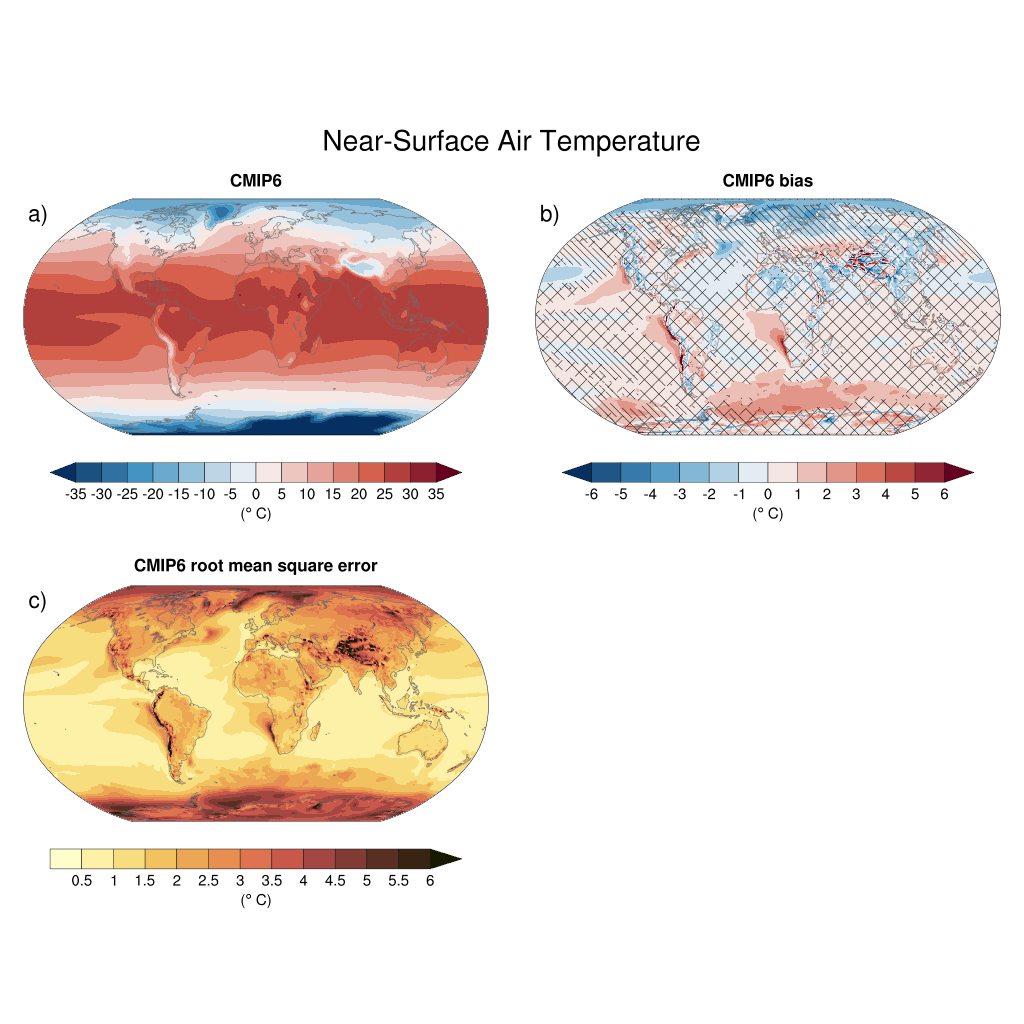
Fig. 276 Figure 3.3: Annual mean near-surface (2 m) air temperature (°C) for the period 1995-2014. (a) Multi-model (ensemble) mean constructed with one realization of the CMIP6 historical experiment from each model. (b) Multi-model mean bias, defined as the difference between the CMIP6 multi-model mean and the climatology of the fifth generation European Centre for Medium-Range Weather Forecasts (ECMWF) atmospheric reanalysis of the global climate (ERA5). (c) Multi-model mean of the root mean square error calculated over all months separately and averaged, with respect to the climatology from ERA5. Uncertainty is represented using the advanced approach: No overlay indicates regions with robust signal, where >=66% of models show change greater than the variability threshold and >=80% of all models agree on sign of change; diagonal lines indicate regions with no change or no robust signal, where <66% of models show a change greater than the variability threshold; crossed lines indicate regions with conflicting signal, where >=66% of models show change greater than the variability threshold and <80% of all models agree on sign of change.#
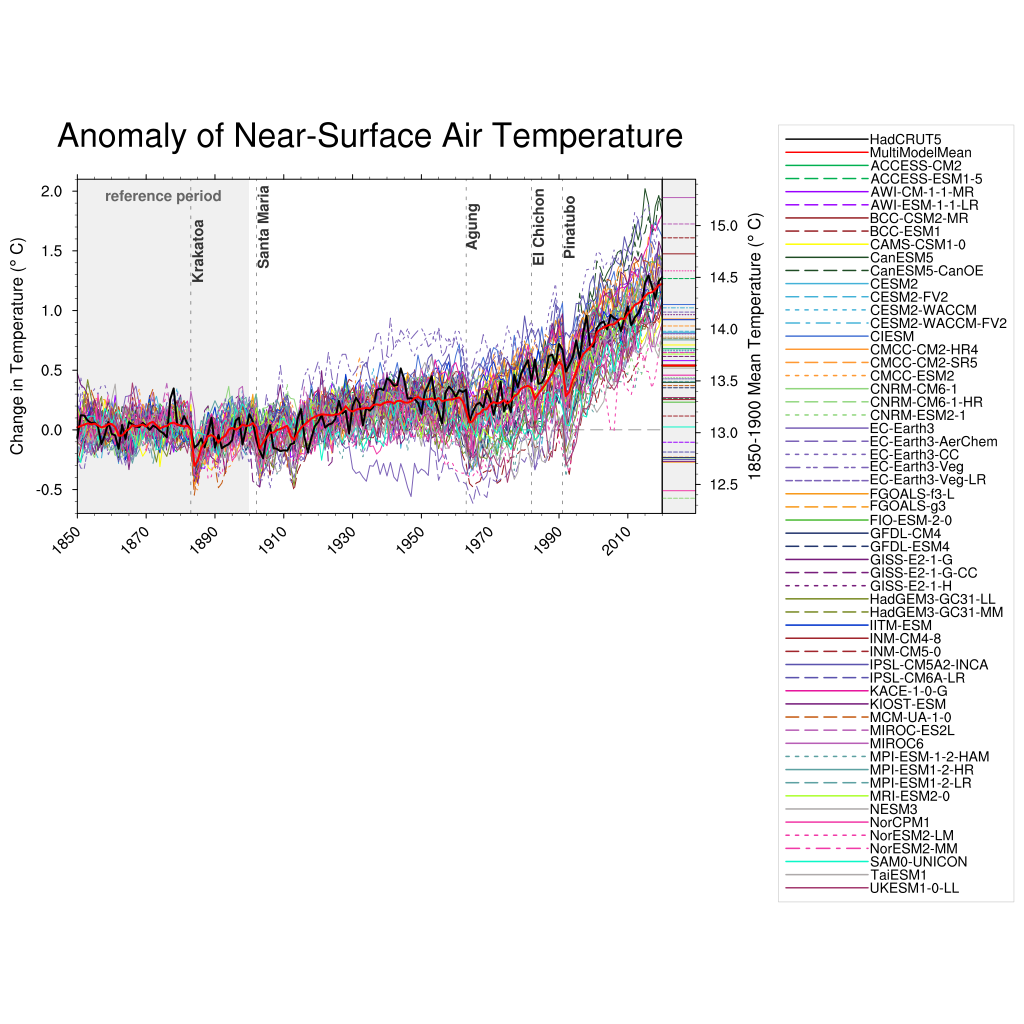
Fig. 277 Figure 3.4a: Observed and simulated time series of the anomalies in annual and global mean surface air temperature (GSAT). All anomalies are differences from the 1850-1900 time-mean of each individual time series. The reference period 1850-1900 is indicated by grey shading. (a) Single simulations from CMIP6 models (thin lines) and the multi-model mean (thick red line). Observational data (thick black lines) are from the Met Office Hadley Centre/Climatic Research Unit dataset (HadCRUT5), and are blended surface temperature (2 m air temperature over land and sea surface temperature over the ocean). All models have been subsampled using the HadCRUT5 observational data mask. Vertical lines indicate large historical volcanic eruptions. Inset: GSAT for each model over the reference period, not masked to any observations.#
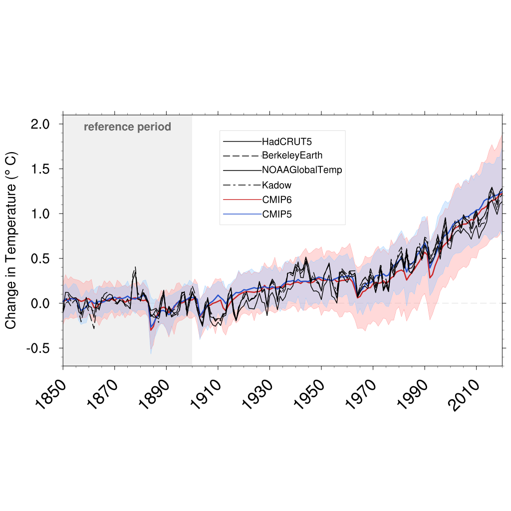
Fig. 278 Figure 3.4b: Observed and simulated time series of the anomalies in annual and global mean surface air temperature (GSAT). All anomalies are differences from the 1850-1900 time-mean of each individual time series. The reference period 1850-1900 is indicated by grey shading. (b) Multi-model means of CMIP5 (blue line) and CMIP6 (red line) ensembles and associated 5th to 95th percentile ranges (shaded regions). Observational data are HadCRUT5, Berkeley Earth, National Oceanic and Atmospheric Administration NOAAGlobalTemp and Kadow et al. (2020). Masking was done as in (a). CMIP6 historical simulations were extended with SSP2-4.5 simulations for the period 2015-2020 and CMIP5 simulations were extended with RCP4.5 simulations for the period 2006-2020. All available ensemble members were used. The multi-model means and percentiles were calculated solely from simulations available for the whole time span (1850-2020).#
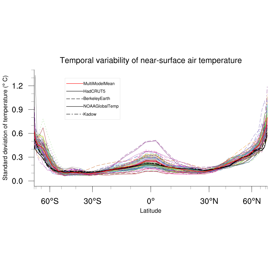
Fig. 279 Figure 3.5: The standard deviation of annually averaged zonal-mean near-surface air temperature. This is shown for four detrended observed temperature datasets (HadCRUT5, Berkeley Earth, NOAAGlobalTemp and Kadow et al. (2020), for the years 1995-2014) and 59 CMIP6 pre-industrial control simulations (one ensemble member per model, 65 years) (after Jones et al., 2013). For line colours see the legend of Figure 3.4. Additionally, the multi-model mean (red) and standard deviation (grey shading) are shown. Observational and model datasets were detrended by removing the least-squares quadratic trend.#
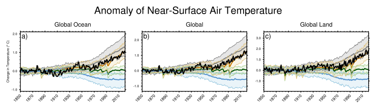
Fig. 280 Figure 3.9: Global, land and ocean annual mean near-surface air temperature anomalies in CMIP6 models and observations. Timeseries are shown for CMIP6 historical anthropogenic and natural (brown) natural-only (green), greenhouse gas only (grey) and aerosol only (blue) simulations (multi-model means shown as thick lines, and shaded ranges between the 5th and 95th percentiles) and for HadCRUT5 (black). All models have been subsampled using the HadCRUT5 observational data mask. Temperature anomalies are shown relative to 1950-2010 for Antarctica and relative to 1850-1900 for other continents. CMIP6 historical simulations are expanded by the SSP2-4.5 scenario simulations. All available ensemble members were used. Regions are defined by Iturbide et al. (2020).#
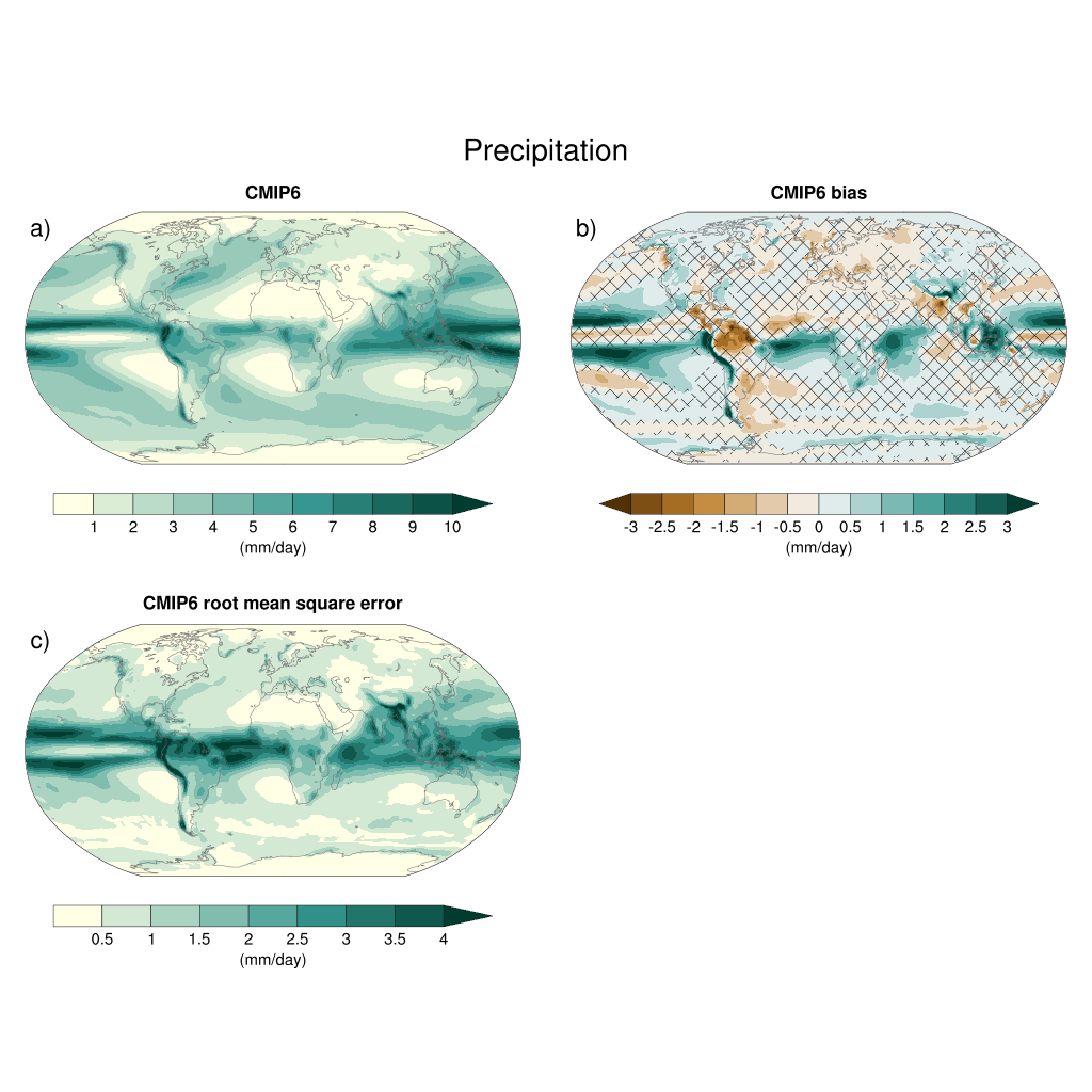
Fig. 281 Figure 3.13: Annual-mean precipitation rate (mm day-1) for the period 1995-2014. (a) Multi-model (ensemble) mean constructed with one realization of the CMIP6 historical experiment from each model. (b) Multi-model mean bias, defined as the difference between the CMIP6 multi-model mean and precipitation analysis from the Global Precipitation Climatology Project (GPCP) version 2.3 (Adler et al., 2003). (c) Multi-model mean of the root mean square error calculated over all months separately and averaged with respect to the precipitation analysis from GPCP version 2.3. Uncertainty is represented using the advanced approach. No overlay indicates regions with robust signal, where >=66% of models show change greater than the variability threshold and >=80% of all models agree on sign of change; diagonal lines indicate regions with no change or no robust signal, where <66% of models show a change greater than the variability threshold; crossed lines indicate regions with conflicting signal, where >=66% of models show change greater than the variability threshold and <80% of all models agree on the sign of change.#
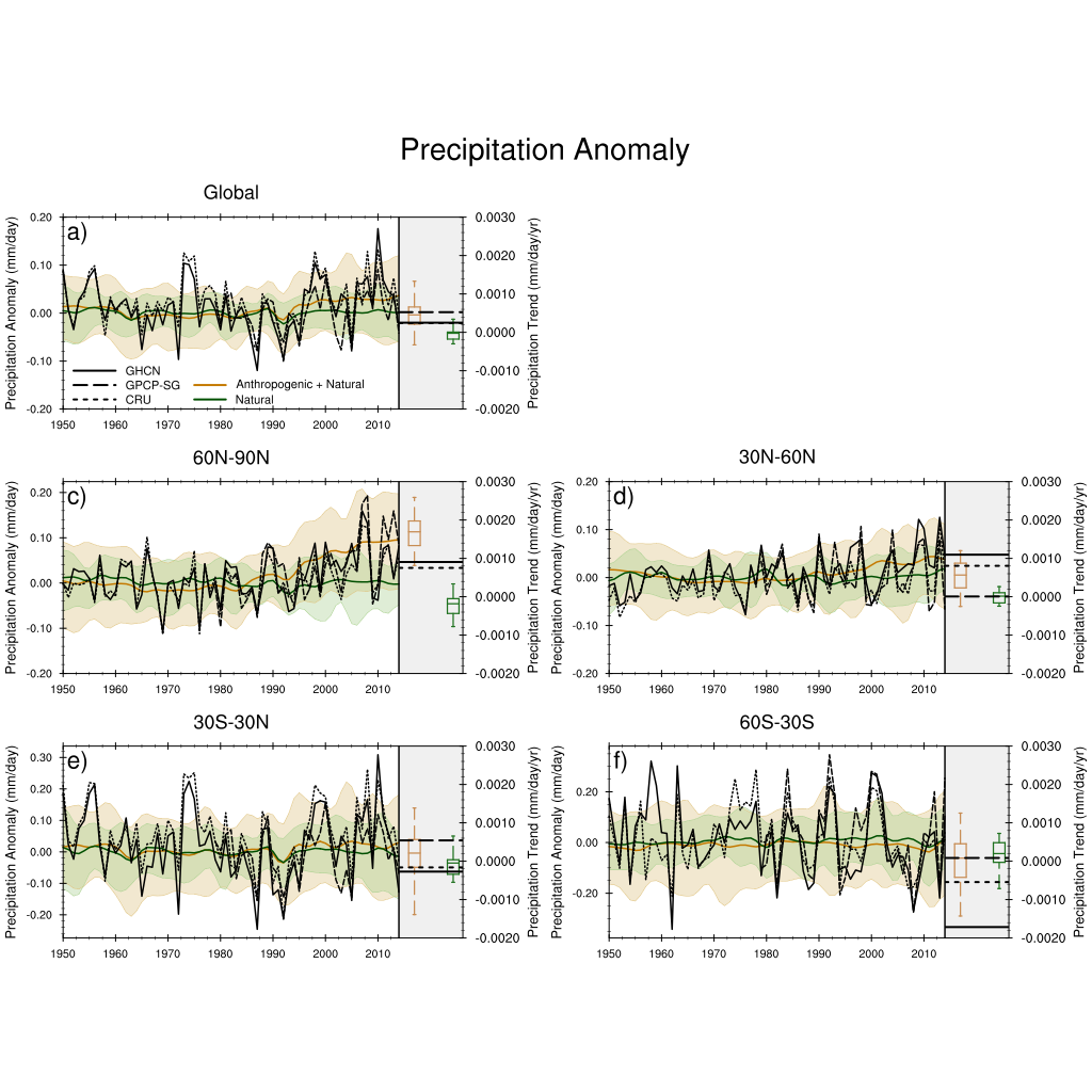
Fig. 282 Figure 3.15: Observed and simulated time series of anomalies in zonal average annual mean precipitation. (a), (c-f) Evolution of global and zonal average annual mean precipitation (mm day-1) over areas of land where there are observations, expressed relative to the base period of 1961-1990, simulated by CMIP6 models (one ensemble member per model) forced with both anthropogenic and natural forcings (brown) and natural forcings only (green). Multi-model means are shown in thick solid lines and shading shows the 5-95% confidence interval of the individual model simulations. The data is smoothed using a low pass filter. Observations from three different datasets are included: gridded values derived from Global Historical Climatology Network (GHCN version 2) station data, updated from Zhang et al. (2007), data from the Global Precipitation Climatology Product (GPCP L3 version 2.3, Adler et al. (2003)) and from the Climate Research Unit (CRU TS4.02, Harris et al. (2014)). Also plotted are boxplots showing interquartile and 5-95% ranges of simulated trends over the period for simulations forced with both anthropogenic and natural forcings (brown) and natural forcings only (blue). Observed trends for each observational product are shown as horizontal lines. Panel (b) shows annual mean precipitation rate (mm day-1) of GHCN version 2 for the years 1950-2014 over land areas used to compute the plots.#
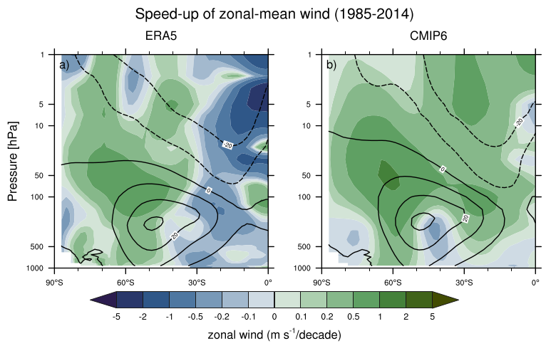
Fig. 283 Figure 3.19: Long-term mean (thin black contours) and linear trend (colour) of zonal mean December-January-February zonal winds from 1985 to 2014 in the Southern Hemisphere. The figure shows (a) ERA5 and (b) the CMIP6 multi-model mean (58 CMIP6 models). The solid contours show positive (westerly) and zero long-term mean zonal wind, and the dashed contours show negative (easterly) long-term mean zonal wind. Only one ensemble member per model is included. Figure is modified from Eyring et al. (2013), their Figure 12.#
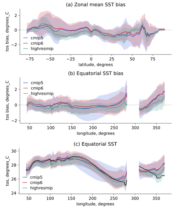
Fig. 284 Figure 3.24: Biases in zonal mean and equatorial sea surface temperature (SST) in CMIP5 and CMIP6 models. CMIP6 (red), CMIP5 (blue) and HighResMIP (green) multi-model mean (a) zonally averaged SST bias; (b) equatorial SST bias; and (c) equatorial SST compared to observed mean SST (black line) for 1979–1999. The inter-model 5th and 95th percentiles are depicted by the respective shaded range. Model climatologies are derived from the 1979–1999 mean of the historical simulations, using one simulation per model. The Hadley Centre Sea Ice and Sea Surface Temperature version 1 (HadISST) observational climatology for 1979–1999 is used as the reference for the error calculation in (a) and (b); and for observations in (c). (The panels were obtained individually and combined together.)#
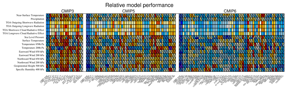
Fig. 285 Figure 3.42a: Relative space-time root-mean-square deviation (RMSD) calculated from the climatological seasonal cycle of the CMIP simulations (1980-1999) compared to observational datasets. A relative performance measure is displayed, with blue shading indicating better and red shading indicating worse performance than the median error of all model results. A diagonal split of a grid square shows the relative error with respect to the reference data set (lower right triangle) and an additional data set (upper left triangle). Reference/additional datasets are from top to bottom in (a): ERA5/NCEP, GPCP-SG/GHCN, CERES-EBAF, CERES-EBAF, CERES-EBAF, CERES-EBAF, JRA-55/ERA5, ESACCI-SST/HadISST, ERA5/NCEP, ERA5/NCEP, ERA5/NCEP, ERA5/NCEP, ERA5/NCEP, ERA5/NCEP, AIRS/ERA5, ERA5/NCEP. White boxes are used when data are not available for a given model and variable. Figure is updated and expanded from Bock et al. (2020).#
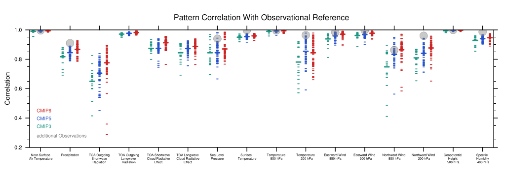
Fig. 286 Figure 3.43 | Centred pattern correlations between models and observations for the annual mean climatology over the period 1980-1999. Results are shown for individual CMIP3 (green), CMIP5 (blue) and CMIP6 (red) models (one ensemble member from each model is used) as short lines, along with the corresponding multi-model ensemble averages (long lines). Correlations are shown between the models and the primary reference observational data set (from left to right: ERA5, GPCP-SG, CERES-EBAF, CERES-EBAF, CERES-EBAF, CERES-EBAF, JRA-55, ESACCI-SST, ERA5, ERA5, ERA5, ERA5, ERA5, ERA5, AIRS, ERA5). In addition, the correlation between the primary reference and additional observational datasets (from left to right: NCEP, GHCN, -, -, -, -, ERA5, HadISST, NCEP, NCEP, NCEP, NCEP, NCEP, NCEP, NCEP, ERA5) are shown (solid grey circles) if available. To ensure a fair comparison across a range of model resolutions, the pattern correlations are computed after regridding all datasets to a resolution of 4° in longitude and 5° latitude.#