Land and ocean components of the global carbon cycle#
Overview#
This recipe reproduces most of the figures of Anav et al. (2013):
Timeseries plot for different regions
Seasonal cycle plot for different regions
Errorbar plot for different regions showing mean and standard deviation
Scatterplot for different regions showing mean vs. interannual variability
3D-scatterplot for different regions showing mean vs. linear trend and the model variability index (MVI) as a third dimension (color coded)
Scatterplot for different regions comparing two variable against each other (cSoil vs. cVeg)
In addition, performance metrics are calculated for all variables using the performance metric diagnostics (see details in Performance metrics for essential climate parameters).
MVI calculation#
The Model variability index (MVI) on a single grid point (calculated in
carbon_cycle/mvi.ncl is defined as
where \(s^M\) and \(s^O\) are the standard deviations of the annual time series on a single grid point of a climate model \(M\) and the reference observation \(O\). In order to get a global or regional result, this index is simple averaged over the respective domain.
In its given form, this equation is prone to small standard deviations close to zero. For example, values of \(s^M = 10^{-5} \mu\) and \(s^O = 10^{-7} \mu\) (where \(\mu\) is the mean of \(s^O\) over all grid cells) results in a MVI of the order of \(10^4\) for this single grid cell even though the two standard deviations are close to zero and negligible compared to other grid cells. Due to the use of the arithmetic mean, a single high value is able to distort the overall MVI.
In the original publication, the maximum MVI is in the order of 10 (for the variable gpp). However, a naive application of the MVI definition yields values over \(10^9\) for some models. Unfortunately, Anav et al. (2013) do not provide an explanation on how to deal with this problem. Nevertheless, this script provides two configuration options to avoid high MVI values, but they are not related to the original paper or any other peer-revied study and should be used with great caution (see User settings in recipe).
Available recipes and diagnostics#
Recipes are stored in recipes/
recipe_anav13jclim.yml
Diagnostics are stored in diag_scripts/
carbon_cycle/main.ncl
carbon_cycle/mvi.ncl
carbon_cycle/two_variables.ncl
perfmetrics/main.ncl
perfmetrics/collect.ncl
User settings in recipe#
Preprocessor
mask_fillvalues: Mask common missing values on different datasets.mask_landsea: Mask land/ocean.regrid: Regridding.weighting_landsea_fraction: Land/ocean fraction weighting.
Script carbon_cycle/main.ncl
region, str: Region to be averaged.legend_outside, bool: Plot legend in a separate file (does not affect errorbar plot and evolution plot)seasonal_cycle_plot, bool: Draw seasonal cycle plot.errorbar_plot, bool: Draw errorbar plot.mean_IAV_plot, bool: Draw Mean (x-axis), IAV (y-axis) plot.evolution_plot, bool: Draw time evolution of a variable comparing a reference dataset to multi-dataset mean; requires ref_dataset in recipe.sort, bool, optional (default:False): Sort dataset in alphabetical order.anav_month, bool, optional (default:False): Conversion of y-axis to PgC/month instead of /year.evolution_plot_ref_dataset, str, optional: Reference dataset for evolution_plot. Required whenevolution_plotisTrue.evolution_plot_anomaly, str, optional (default:False): Plot anomalies in evolution plot.evolution_plot_ignore, list, optional: Datasets to ignore in evolution plot.evolution_plot_volcanoes, bool, optional (default:False): Turns on/off lines of volcano eruptions in evolution plot.evolution_plot_color, int, optional (default:0): Hue of the contours in the evolution plot.ensemble_name, string, optional: Name of ensemble for use in evolution plot legend
Script carbon_cycle/mvi.ncl
region, str: Region to be averaged.reference_dataset, str: Reference dataset for the MVI calculation specified for each variable seperately.mean_time_range, list, optional: Time period over which the mean is calculated (if not given, use whole time span).trend_time_range, list, optional: Time period over which the trend is calculated (if not given, use whole time span).mvi_time_range, list, optional: Time period over which the MVI is calculated (if not given, use whole time span).stddev_threshold, float, optional (default:1e-2): Threshold to ignore low standard deviations (relative to the mean) in the MVI calculations. See also MVI calculation.mask_below, float, optional: Threshold to mask low absolute values (relative to the mean) in the input data (not used by default). See also MVI calculation.
Script carbon_cycle/two_variables.ncl
region, str: Region to be averaged.
Script perfmetrics/main.ncl
Script perfmetrics/collect.ncl
Variables#
tas (atmos, monthly, longitude, latitude, time)
pr (atmos, monthly, longitude, latitude, time)
nbp (land, monthly, longitude, latitude, time)
gpp (land, monthly, longitude, latitude, time)
lai (land, monthly, longitude, latitude, time)
cveg (land, monthly, longitude, latitude, time)
csoil (land, monthly, longitude, latitude, time)
tos (ocean, monthly, longitude, latitude, time)
fgco2 (ocean, monthly, longitude, latitude, time)
Observations and reformat scripts#
CRU (tas, pr)
JMA-TRANSCOM (nbp, fgco2)
MTE (gpp)
LAI3g (lai)
NDP (cveg)
HWSD (csoil)
HadISST (tos)
References#
Anav, A. et al.: Evaluating the land and ocean components of the global carbon cycle in the CMIP5 Earth System Models, J. Climate, 26, 6901-6843, doi: 10.1175/JCLI-D-12-00417.1, 2013.
Example plots#
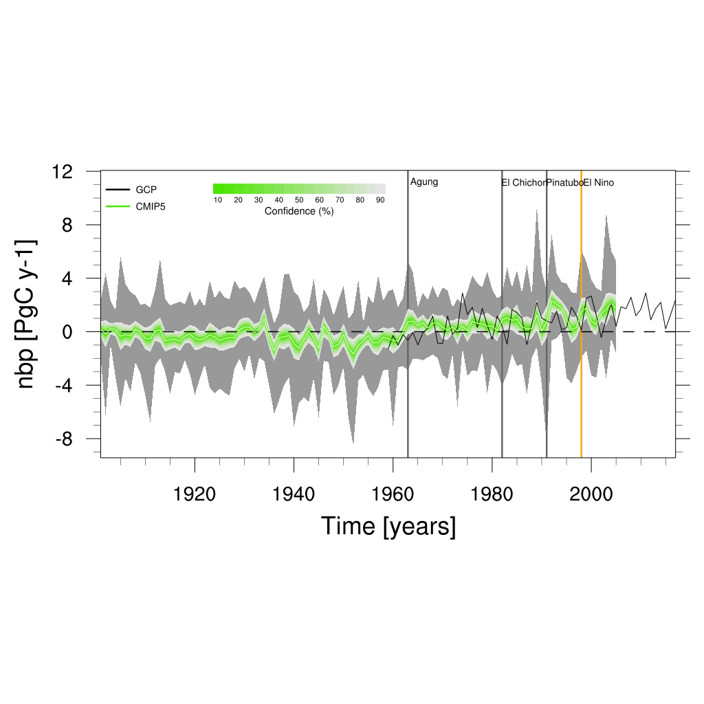
Fig. 330 Time series of global net biome productivity (NBP) over the period 1901-2005. Similar to Anav et al. (2013), Figure 5.#
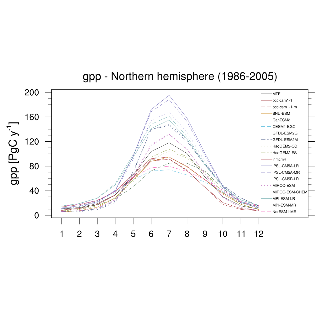
Fig. 331 Seasonal cycle plot for nothern hemisphere gross primary production (GPP) over the period 1986-2005. Similar to Anav et al. (2013), Figure 9.#
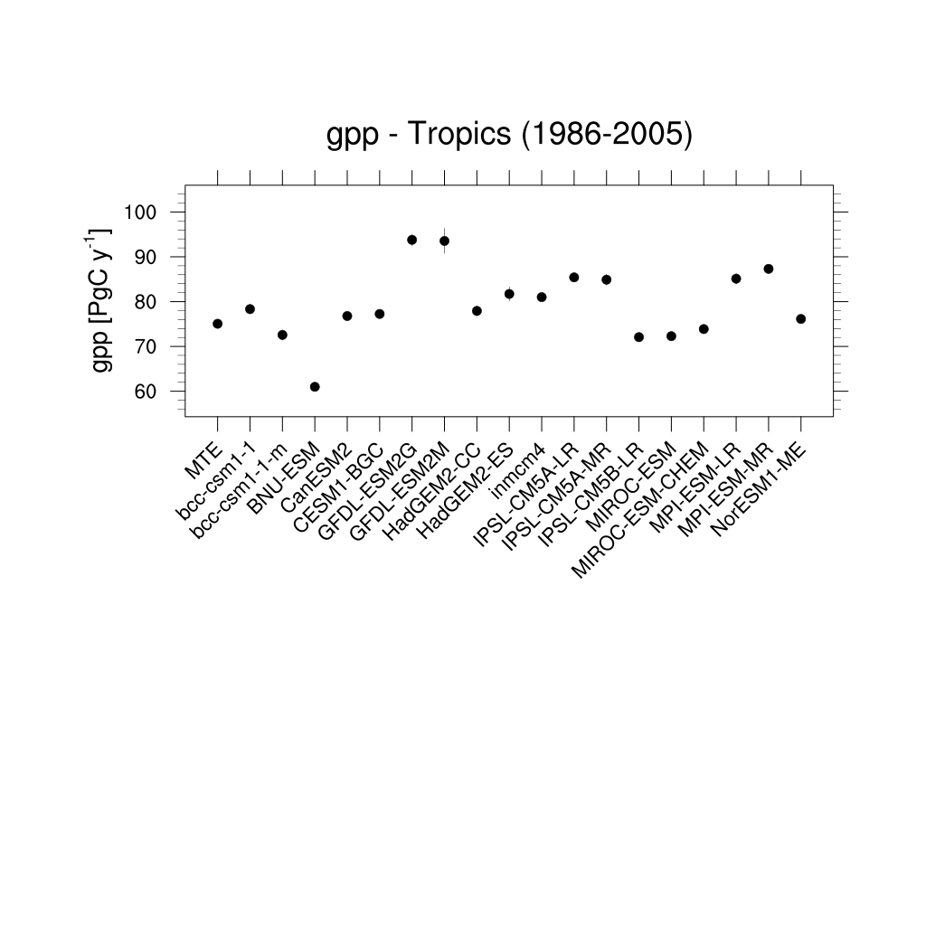
Fig. 332 Errorbar plot for tropical gross primary production (GPP) over the period 1986-2005.#
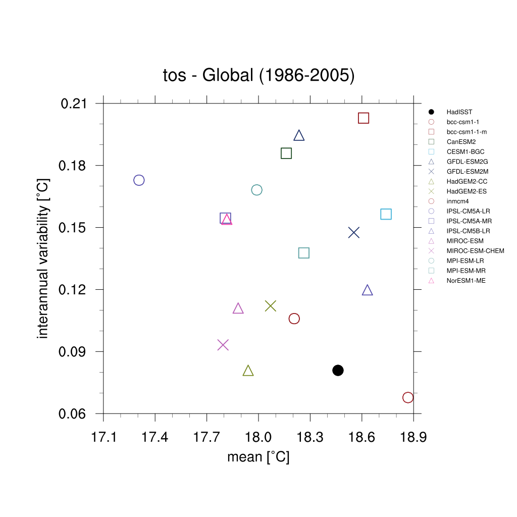
Fig. 333 Scatterplot for interannual variability and mean of global sea surface temperature (TOS) over the period 1986-2005.#
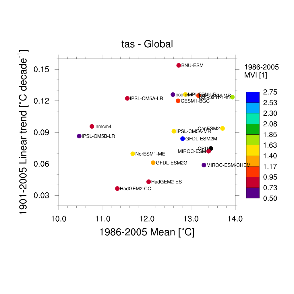
Fig. 334 Scatterplot for multiyear average of 2m surface temperature (TAS) in x axis, its linear trend in y axis, and MVI. Similar to Anav et al. (2013) Figure 1 (bottom).#
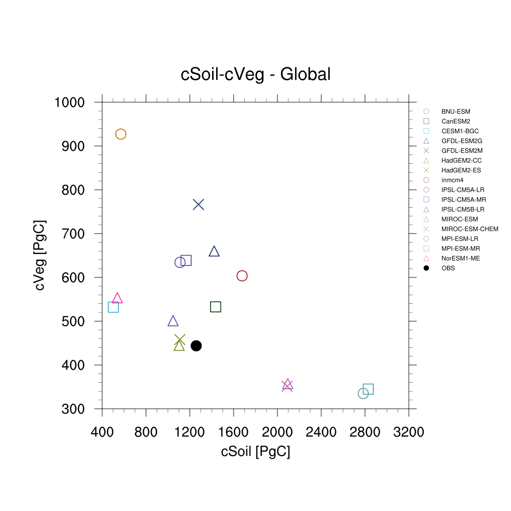
Fig. 335 Scatterplot for vegetation carbon content (cVeg) and soil carbon content (cSoil) over the period 1986-2005. Similar to Anav et al. (2013), Figure 12.#
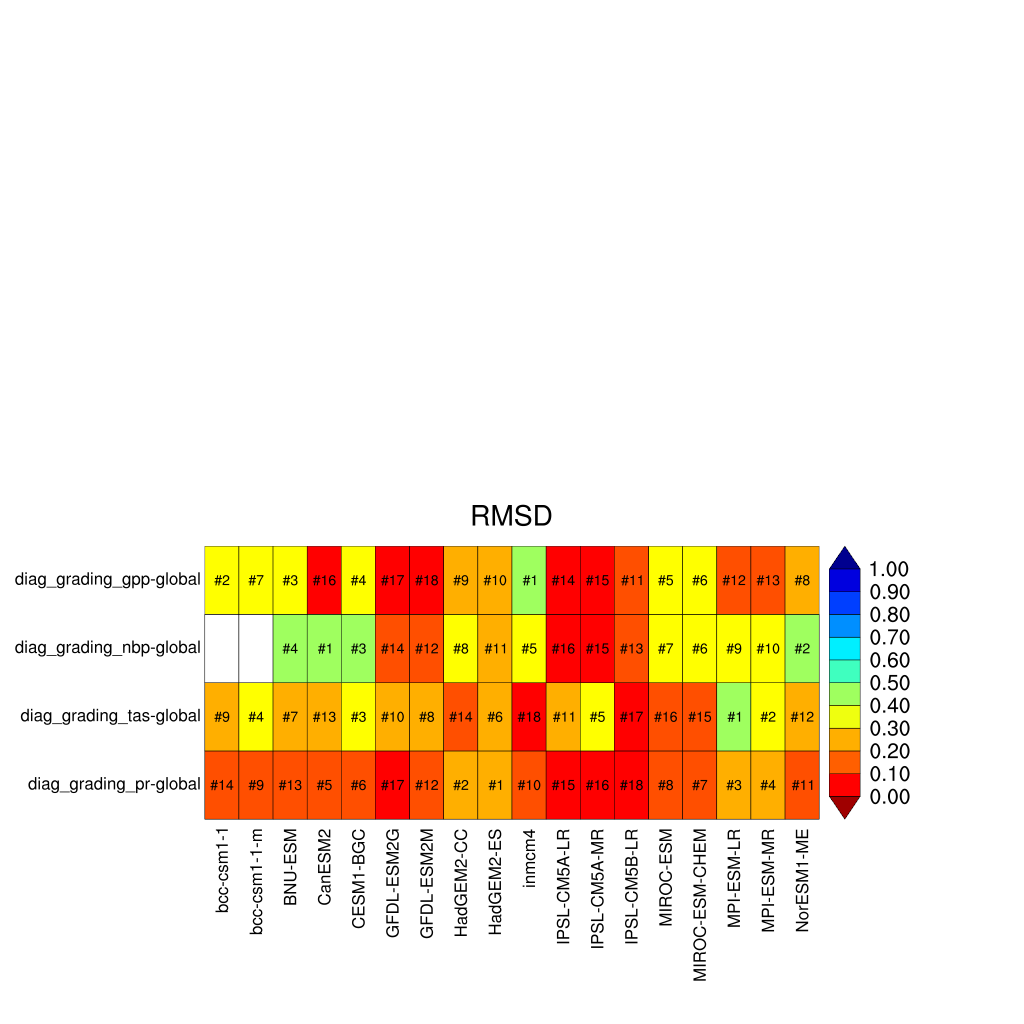
Fig. 336 Performance metrics plot for carbon-cycle-relevant diagnostics.#