Model Benchmarking

Overview

These recipes and diagnostics are based on recipe_monitor that allow plotting arbitrary preprocessor output, i.e., arbitrary variables from arbitrary datasets. An extension of these diagnostics is used to benchmark a model simulation with other datasets (e.g. CMIP6). The benchmarking features are described in Lauer et al..

Available recipes and diagnostics

Recipes are stored in recipes/model_evaluation

• recipe_model_benchmarking_annual_cycle.yml

• recipe_model_benchmarking_boxplots.yml

• recipe_model_benchmarking_diurnal_cycle.yml

• recipe_model_benchmarking_maps.yml

• recipe_model_benchmarking_timeseries.yml

• recipe_model_benchmarking_zonal.yml

Diagnostics are stored in diag_scripts/monitor/

• multi_datasets.py: Monitoring diagnostic to show multiple datasets in one plot (incl. biases).

Recipe settings

See multi_datasets.py for a list of all possible configuration options that can be specified in the recipe.

Note

Please note that exactly one dataset (the dataset to be benchmarked) needs to specify the facet benchmark_dataset: true in the dataset entry of the recipe. For line plots (i.e. annual cycle, diurnal cycle, time series), it is recommended, to specify a particular line color and line style in the scripts section of the recipe for the dataset to be benchmarked (benchmark_dataset: true) so that this dataset is easy to identify in the plot. In the example below, MIROC6 is the dataset to be benchmarked and ERA5 is used as a reference dataset.

scripts:
  allplots:
    script: monitor/multi_datasets.py
    plot_folder: '{plot_dir}'
    plot_filename: '{plot_type}_{real_name}_{mip}'
    group_variables_by: variable_group
    facet_used_for_labels: alias
    plots:
      diurnal_cycle:
        annual_mean_kwargs: false
        legend_kwargs:
          loc: upper right
        plot_kwargs:
          'MIROC6':
            color: red
            label: '{alias}'
            linestyle: '-'
            linewidth: 2
            zorder: 4
          ERA5:
            color: black
            label: '{dataset}'
            linestyle: '-'
            linewidth: 2
            zorder: 3
          MultiModelPercentile10:
            color: gray
            label: '{dataset}'
            linestyle: '--'
            linewidth: 1
            zorder: 2
          MultiModelPercentile90:
            color: gray
            label: '{dataset}'
            linestyle: '--'
            linewidth: 1
            zorder: 2
          default:
            color: lightgray
            label: null
            linestyle: '-'
            linewidth: 1
            zorder: 1

Variables

Any, but the variables’ number of dimensions should match the ones expected by each plot.

References

• Lauer, A., L. Bock, B. Hassler, P. Jöckel, L. Ruhe, and M. Schlund: Monitoring and benchmarking Earth System Model simulations with ESMValTool v2.12.0, EGUsphere [preprint], https://doi.org/10.5194/egusphere-2024-1518, 2024.

Example plots

Fig. 2 (Left) Multi-year global mean (2000-2004) of the seasonal cycle of near-surface temperature in K from a simulation of MIROC6 and the reference dataset HadCRUT5 (black). The thin gray lines show individual CMIP6 models used for comparison, the dashed gray lines show the 10% and 90% percentiles of these CMIP6 models. (Right) same as (left) but for area-weighted RMSE of near-surface temperature. The light blue shading shows the range of the 10% to 90% percentiles of RMSE values from the ensemble of CMIP6 models used for comparison. Created with recipe_model_benchmarking_annual_cycle.yml.

Fig. 3 (Left) Global area-weighted RMSE (smaller=better), (middle) weighted Pearson’s correlation coefficient (higher=better) and (right) weighted Earth mover’s distance (smaller=better) of the geographical pattern of 5-year means of different variables from a simulation of MIROC6 (red cross) in comparison to the CMIP6 ensemble (boxplot). Reference datasets for calculating the three metrics are: near-surface temperature (tas): HadCRUT5, surface temperature (ts): HadISST, precipitation (pr): GPCP-SG, air pressure at sea level (psl): ERA5, shortwave (rsut) longwave (rlut) radiative fluxes at TOA and shortwave (swcre) and longwave (lwcre) cloud radiative effects: CERES-EBAF. Each box indicates the range from the first quartile to the third quartile, the vertical lines show the median, and the whiskers the minimum and maximum values, excluding the outliers. Outliers are defined as being outside 1.5 times the interquartile range. Created with recipe_model_benchmarking_boxplots.yml.

Fig. 4 Area-weighted RMSE of the annual mean diurnal cycle (year 2000) of precipitation averaged over the tropical ocean (ocean grid cells in the latitude belt 30°S to 30°N) from a simulation of MIROC6 averaged compared with ERA5 data (black). The light blue shading shows the range of the 10% to 90% percentiles of RMSE values from the ensemble of CMIP6 models used for comparison. Created with recipe_benchmarking_diurnal_cycle.yml.

Fig. 5 5-year annual mean (2000-2004) area-weighted RMSE of the precipitation rate in mm day-1 from a simulation of MIROC6 compared with GPCP-SG data. The stippled areas mask grid cells where the RMSE is smaller than the 90% percentile of RMSE values from an ensemble of CMIP6 models. Created with recipe_model_benchmarking_maps.yml

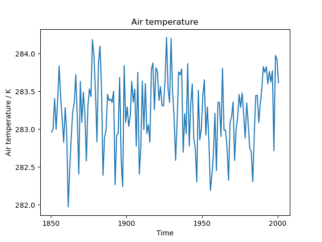
Fig. 6 (Left) Time series from 2000 through 2014 of global average monthly mean temperature anomalies (reference period 2000-2009) of the near-surface temperature in K from a simulation of MIROC6 (red) and the reference dataset HadCRUT5 (black). The thin gray lines show individual CMIP6 models used for comparison, the dashed gray lines show the 10% and 90% percentiles of these CMIP6 models. (Right) same as (left) but for area-weighted RMSE of the near-surface air temperature. The light blue shading shows the range of the 10% to 90% percentiles of RMSE values from the ensemble of CMIP6 models used for comparison. Created with recipe_model_benchmarking_timeseries.yml.

Fig. 7 5-year annual mean bias (2000-2004) of the zonally averaged temperature in K from a historical simulation of MIROC6 compared with ERA5 reanalysis data. The stippled areas mask grid cells where the absolute BIAS (\(|BIAS|\)) is smaller than the maximum of the absolute 10% (\(|p10|\)) and the absolute 90% (\(|p90|\)) percentiles from an ensemble of CMIP6 models, i.e. \(|BIAS| \geq max( |p10|, |p90|)\). Created with recipe_model_benchmarking_zonal.yml.