Sea Ice#
Overview#
The sea ice diagnostics include:
time series of Arctic and Antarctic sea ice area and extent (calculated as the total area (km2) of grid cells with sea ice concentrations (sic) of at least 15%).
ice extent trend distributions for the Arctic in September and the Antarctic in February.
calculation of year of near disappearance of Arctic sea ice
scatter plots of (a) historical trend in September Arctic sea ice extent (SSIE) vs historical long-term mean SSIE; (b) historical SSIE mean vs 1st year of disappearance (YOD) RCP8.5; (c) historical SSIE trend vs YOD RCP8.5.
Available recipes and diagnostics#
Recipes are stored in recipes/
recipe_seaice.yml
Diagnostics are stored in diag_scripts/seaice/
seaice_aux.ncl: contains functions for calculating sea ice area or extent from sea ice concentration and first year of disappearance
seaice_ecs.ncl: scatter plots of mean/trend of historical September Arctic sea ice extent vs 1st year of disappearance (RCP8.5) (similar to IPCC AR5 Chapter 12, Fig. 12.31a)
seaice_trends.ncl: calculates ice extent trend distributions (similar to IPCC AR5 Chapter 9, Fig. 9.24c/d)
seaice_tsline.ncl: creates a time series line plots of total sea ice area and extent (accumulated) for northern and southern hemispheres with optional multi-model mean and standard deviation. One value is used per model per year, either annual mean or the mean value of a selected month (similar to IPCC AR5 Chapter 9, Fig. 9.24a/b)
seaice_yod.ncl: calculation of year of near disappearance of Arctic sea ice
User settings in recipe#
Script seaice_ecs.ncl
Required settings (scripts)
hist_exp: name of historical experiment (string)
month: selected month (1, 2, …, 12) or annual mean (“A”)
rcp_exp: name of RCP experiment (string)
region: region to be analyzed ( “Arctic” or “Antarctic”)
Optional settings (scripts)
fill_pole_hole: fill observational hole at North pole (default: False)
styleset: color style (e.g. “CMIP5”)
Optional settings (variables)
reference_dataset: reference dataset
Script seaice_trends.ncl
Required settings (scripts)
month: selected month (1, 2, …, 12) or annual mean (“A”)
region: region to be analyzed ( “Arctic” or “Antarctic”)
Optional settings (scripts)
fill_pole_hole: fill observational hole at North pole, Default: False
Optional settings (variables)
ref_model: array of references plotted as vertical lines
Script seaice_tsline.ncl
Required settings (scripts)
region: Arctic, Antarctic
month: annual mean (A), or month number (3 = March, for Antarctic; 9 = September for Arctic)
Optional settings (scripts)
styleset: for plot_type cycle only (cmip5, cmip6, default)
multi_model_mean: plot multi-model mean and standard deviation (default: False)
EMs_in_lg: create a legend label for individual ensemble members (default: False)
fill_pole_hole: fill polar hole (typically in satellite data) with sic = 1 (default: False)
Script seaice_yod.ncl
Required settings (scripts)
month: selected month (1, 2, …, 12) or annual mean (“A”)
region: region to be analyzed ( “Arctic” or “Antarctic”)
Optional settings (scripts)
fill_pole_hole: fill observational hole at North pole, Default: False
wgt_file: netCDF containing pre-determined model weights
Optional settings (variables)
ref_model: array of references plotted as vertical lines
Variables#
sic (ocean-ice, monthly mean, longitude latitude time)
areacello (fx, longitude latitude)
Observations and reformat scripts#
Note: (1) obs4MIPs data can be used directly without any preprocessing; (2) use `esmvaltool data info DATASET` or see headers of cmorization scripts (in esmvaltool/cmorizers/data/formatters/datasets/) for non-obs4MIPs data for download instructions.
HadISST (sic - esmvaltool/cmorizers/data/formatters/datasets/hadisst.ncl)
References#
Massonnet, F. et al., The Cryosphere, 6, 1383-1394, doi: 10.5194/tc-6-1383-2012, 2012.
Stroeve, J. et al., Geophys. Res. Lett., 34, L09501, doi:10.1029/2007GL029703, 2007.
Example plots#
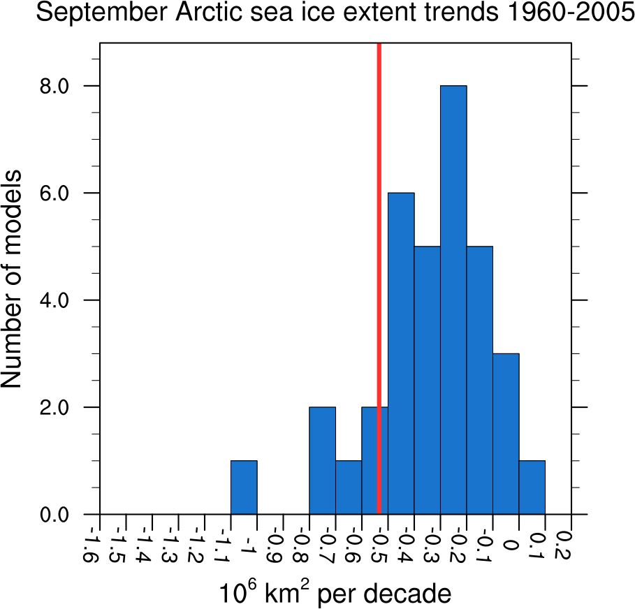
Fig. 394 Sea ice extent trend distribution for the Arctic in September (similar to IPCC AR5 Chapter 9, Fig. 9.24c). [seaice_trends.ncl]#
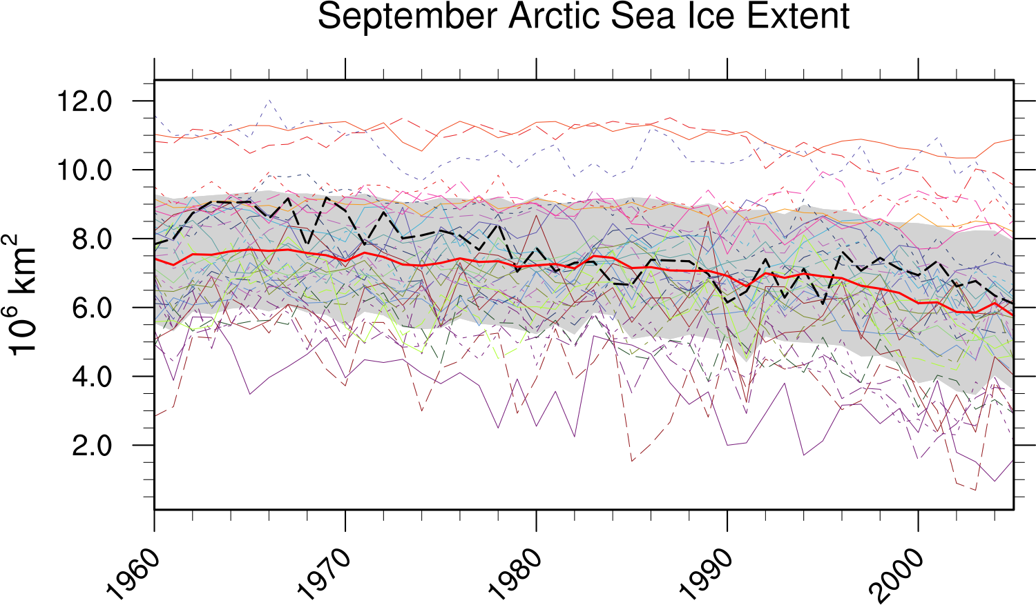
Fig. 395 Time series of total sea ice area and extent (accumulated) for the Arctic in September including multi-model mean and standard deviation (similar to IPCC AR5 Chapter 9, Fig. 9.24a). [seaice_tsline.ncl]#
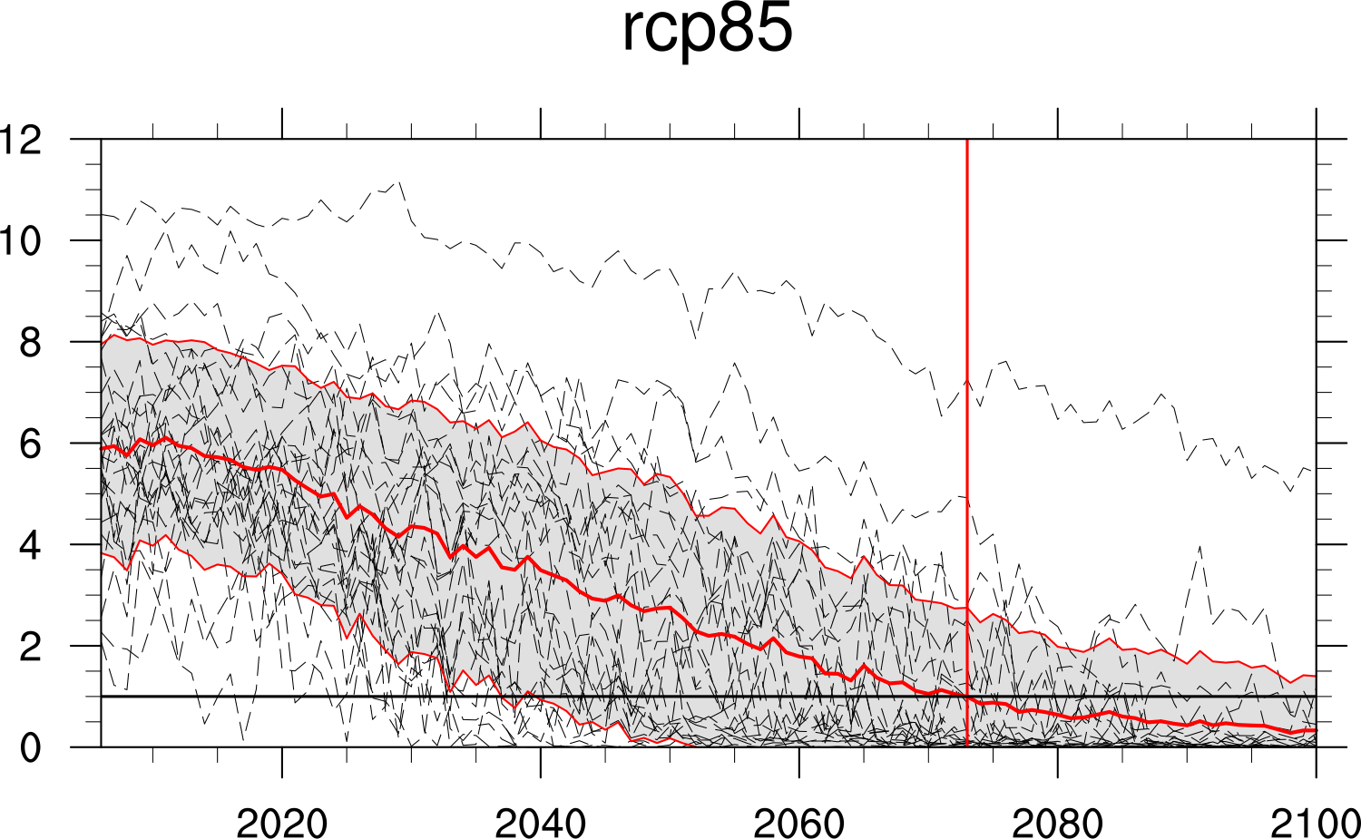
Fig. 396 Time series of September Arctic sea ice extent for individual CMIP5 models, multi-model mean and multi-model standard deviation, year of disappearance (similar to IPCC AR5 Chapter 12, Fig. 12.31e). [seaice_yod.ncl]#
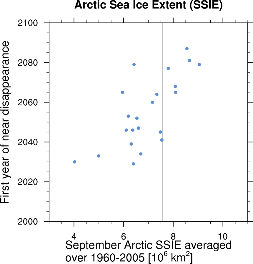
Fig. 397 Scatter plot of mean historical September Arctic sea ice extent vs 1st year of disappearance (RCP8.5) (similar to IPCC AR5 Chapter 12, Fig. 12.31a). [seaice_ecs.ncl]#