Clouds#
Overview#
Four recipes are available to evaluate cloud climatologies from CMIP models.
recipe_clouds_bias.yml computes climatologies and creates map plots of multi-model mean, mean bias, absolute bias and relative bias of a given variable. Similar to IPCC AR5 (ch. 9) fig. 9.2 a/b/c (Flato et al., 2013).
recipe_clouds_ipcc.yml computes multi-model mean bias and zonal means of the clouds radiative effect (shortwave, longwave and net). Similar to IPCC AR5 (ch. 9) fig. 9.5 (Flato et al., 2013).
Recipe recipe_lauer13jclim.yml computes the climatology and interannual variability of climate relevant cloud variables such as cloud radiative forcing (CRE), liquid water path (lwp), cloud amount (clt), and total precipitation (pr) reproducing some of the evaluation results of Lauer and Hamilton (2013). The recipe includes a comparison of the geographical distribution of multi-year average cloud parameters from individual models and the multi-model mean with satellite observations. Taylor diagrams are generated that show the multi-year annual or seasonal average performance of individual models and the multi-model mean in reproducing satellite observations. The diagnostic also facilitates the assessment of the bias of the multi-model mean and zonal averages of individual models compared with satellite observations. Interannual variability is estimated as the relative temporal standard deviation from multi-year timeseries of data with the temporal standard deviations calculated from monthly anomalies after subtracting the climatological mean seasonal cycle. Note that the satellite observations used in the original recipe (UWisc) is not maintained anymore and has been superseeded by MAC-LWP (Elsaesser et al., 2017). We recommend using MAC-LWP.
Recipe family recipe_lauer22jclim_*.yml is an extension of recipe_lauer13jclim.yml for evaluation of cloud radiative forcing (CRE), liquid water path (lwp), ice water path (clivi), total cloud amount (clt), cloud liquid water content (clw), cloud ice water content (cli), cloud fraction (cl) and water vapor path (prw) from CMIP6 models in comparison to CMIP5 results and satellite observations. Wherever possible, the diagnostics use multi-observational products as reference datasets. The recipe family reproduces all figures from Lauer et al. (2023): maps of the geographical distribution of multi-year averages, Taylor diagrams for multi-year annual averages, temporal variability, seasonal cycle amplitude, cloud ice fraction as a function of temperature, zonal means of 3-dim cloud liquid/ice content and cloud fraction, matrices of cloud cover and total cloud water path as a function of SST and 500 hPa vertical velocity, shortwave CRE and total cloud water path binned by total cloud cover and pdfs of total cloud cover for selected regions.
Available recipes and diagnostics#
Recipes are stored in recipes/clouds
recipe_clouds_bias.yml
recipe_clouds_ipcc.yml
recipe_lauer13jclim.yml
recipe_lauer22jclim_*.yml (* = fig1_clim_amip, fig1_clim, fig2_taylor_amip, fig2_taylor, fig3-4_zonal, fig5_lifrac, fig6_interannual, fig7_seas, fig8_dyn, fig9-11ab_scatter, fig9-11c_pdf)
Diagnostics are stored in diag_scripts/clouds/
clouds.ncl: global maps of (multi-year) annual means including multi-model mean
clouds_bias.ncl: global maps of the multi-model mean and the multi-model mean bias
clouds_dyn_matrix.ncl: cloud properties by dynamical regime (SST, omega500)
clouds_interannual.ncl: global maps of the interannual variability
clouds_ipcc.ncl: global maps of multi-model mean minus observations + zonal averages of individual models, multi-model mean and observations
clouds_lifrac_scatter.ncl: cloud liquid water fraction as a function of temperature
clouds_lifrac_scatter_postproc.ncl: additional plots and diagnostics using the output of clouds_lifrac_scatter.ncl for given CMIP5/CMIP6 model pairs
clouds_pdf.ncl: pdf of cloud parameters
clouds_seasonal_cycle.ncl: seasonal cycle amplitude
clouds_taylor.ncl: Taylor diagrams as in Lauer and Hamilton (2013)
clouds_taylor_double.ncl: Taylor diagrams as in Lauer et al. (2023)
clouds_zonal.ncl: zonal means of 3-dim variables
User settings in recipe#
Script clouds.ncl
Required settings (scripts)
none
Optional settings (scripts)
embracesetup: true = 2 plots per line, false = 4 plots per line (default)
explicit_cn_levels: explicit contour levels (array)
extralegend: plot legend(s) to extra file(s)
filename_add: optionally add this string to plot filesnames
multiobs_exclude: list of observational datasets to be excluded when calculating uncertainty estimates from multiple observational datasets (see also multiobs_uncertainty)
multiobs_uncertainty: calculate uncertainty estimates from multiple observational datasets (true, false); by default, all “obs”, “obs6”, “obs4mips” and “native6” datasets are used; any of such datasets can be explicitly excluded when also specifying “multiobs_exclude”
panel_labels: label individual panels (true, false)
PanelTop: manual override for “@gnsPanelTop” used by panel plot(s)
projection: map projection for plotting (default = “CylindricalEquidistant”)
showdiff: calculate and plot differences model - reference (default = false)
showyears: add start and end years to the plot titles (default = false)
rel_diff: if showdiff = true, then plot relative differences (%) (default = False)
ref_diff_min: lower cutoff value in case of calculating relative differences (in units of input variable)
region: show only selected geographic region given as latmin, latmax, lonmin, lonmax
timemean: time averaging - “seasonal” = DJF, MAM, JJA, SON), “annual” = annual mean
treat_var_as_error: treat variable as error when averaging (true, false); true: avg = sqrt(mean(var*var)), false: avg = mean(var)
var: short_name of variable to process (default = “” - use first variable in variable list)
Required settings (variables)
none
Optional settings (variables)
long_name: variable description
reference_dataset: reference dataset; REQUIRED when calculating differences (showdiff = True)
units: variable units (for labeling plot only)
Color tables
variable “lwp”: diag_scripts/shared/plot/rgb/qcm3.rgb
Script clouds_bias.ncl
Required settings (scripts)
none
Optional settings (scripts)
plot_abs_diff: additionally also plot absolute differences (true, false)
plot_rel_diff: additionally also plot relative differences (true, false)
projection: map projection, e.g., Mollweide, Mercator
timemean: time averaging, i.e. “seasonalclim” (DJF, MAM, JJA, SON), “annualclim” (annual mean)
Required settings (variables)*
reference_dataset: name of reference datatset
Optional settings (variables)
long_name: description of variable
Color tables
variable “tas”: diag_scripts/shared/plot/rgb/ipcc-tas.rgb, diag_scripts/shared/plot/rgb/ipcc-tas-delta.rgb
variable “pr-mmday”: diag_scripts/shared/plots/rgb/ipcc-precip.rgb, diag_scripts/shared/plot/rgb/ipcc-precip-delta.rgb
Script clouds_dyn_matrix.ncl
Required settings (scripts)
var_x: short name of variable on x-axis
var_y: short name of variable on y-axis
var_z: short name of variable to be binned
xmin: min x value for generating x bins
xmax: max x value for generating x bins
ymin: min y value for generating y bins
ymax: max y value for generating y bins
Optional settings (scripts)
clevels: explicit values for probability labelbar (array)
filename_add: optionally add this string to plot filesnames
nbins: number of equally spaced bins (var_x), default = 100
sidepanels: show/hide side panels (default = False)
xlabel: label overriding variable name for x-axis (e.g. SST)
ylabel: label overriding variable name for y-axis (e.g. omega500)
zdmin: min z value for labelbar (difference plots)
zdmax: max z value for labelbar (difference plots)
zmin: min z value for labelbar
zmax: max z value for labelbar
Required settings (variables)
Optional settings (variables)
reference_dataset: reference dataset
Script clouds_interannual.ncl
Required settings (scripts)
none
Optional settings (scripts)
colormap: e.g., WhiteBlueGreenYellowRed, rainbow
epsilon: “epsilon” value to be replaced with missing values
explicit_cn_levels: use these contour levels for plotting
filename_add: optionally add this string to plot filesnames
projection: map projection, e.g., Mollweide, Mercator
var: short_name of variable to process (default = “” - use first variable in variable list)
Required settings (variables)
none
Optional settings (variables)
long_name: description of variable
reference_dataset: name of reference datatset
Script clouds_ipcc.ncl
Required settings (scripts)
none
Optional settings (scripts)
explicit_cn_levels: contour levels
highlight_dataset: name of dataset to highlight (default = “MultiModelMean”)
mask_ts_sea_ice: true = mask T < 272 K as sea ice (only for variable “ts”); false = no additional grid cells masked for variable “ts”
projection: map projection, e.g., Mollweide, Mercator
styleset: style set for zonal mean plot (“CMIP5”, “DEFAULT”)
timemean: time averaging, i.e. “seasonalclim” (DJF, MAM, JJA, SON), “annualclim” (annual mean)
valid_fraction: used for creating sea ice mask (mask_ts_sea_ice = true): fraction of valid time steps required to mask grid cell as valid data
Required settings (variables)
reference_dataset: name of reference data set
Optional settings (variables)
long_name: description of variable
units: variable units
Color tables
variables “pr”, “pr-mmday”: diag_scripts/shared/plot/rgb/ipcc-precip-delta.rgb
Script clouds_lifrac_scatter.ncl
Required settings (scripts)
none
Optional settings (scripts)
filename_add: optionally add this string to plot filesnames
min_mass: minimum cloud condensate (same units as clw, cli)
mm_mean_median: calculate multi-model mean and meadian
nbins: number of equally spaced bins (ta (x-axis)), default = 20
panel_labels: label individual panels (true, false)
PanelTop: manual override for “@gnsPanelTop” used by panel plot(s)s
Required settings (variables)
Optional settings (variables)
reference_dataset: reference dataset
Script clouds_lifrac_scatter_postproc.ncl
Required settings (scripts)
models: array of CMIP5/CMIP6 model pairs to be compared
refname: name of reference dataset
Optional settings (scripts)
nbins: number of bins used by clouds_lifrac_scatter.ncl (default = 20)
reg: region (string) (default = “”)
t_int: array of temperatures for printing additional diagnostics
Required settings (variables)
none
Optional settings (variables)
none
Script clouds_pdf.ncl
Required settings (scripts)
xmin: min value for bins (x axis)
xmax: max value for bins (y axis)
Optional settings (scripts)
filename_add: optionally add this string to output filenames
plot_average: show average frequency per bin
region: show only selected geographic region given as latmin, latmax, lonmin, lonmax
styleset: “CMIP5”, “DEFAULT”
ymin: min value for frequencies (%) (y axis)
ymax: max value for frequencies (%) (y axis)
Required settings (variables)
Optional settings (variables)
reference_dataset: reference dataset
Script clouds_seasonal_cycle.ncl
Required settings (scripts)
none
Optional settings (scripts)
colormap: e.g., WhiteBlueGreenYellowRed, rainbow
epsilon: “epsilon” value to be replaced with missing values
explicit_cn_levels: use these contour levels for plotting
filename_add: optionally add this string to plot filesnames
projection: map projection, e.g., Mollweide, Mercator
showyears: add start and end years to the plot titles (default = false)
var: short_name of variable to process (default = “” i.e. use first variable in variable list)
Required settings (variables)
Optional settings (variables)
long_name: description of variable
reference_dataset: name of reference dataset
Script clouds_taylor.ncl
Required settings (scripts)
none
Optional settings (scripts)
embracelegend: false (default) = include legend in plot, max. 2 columns with dataset names in legend; true = write extra file with legend, max. 7 dataset names per column in legend, alternative observational dataset(s) will be plotted as a red star and labeled “altern. ref. dataset” in legend (only if dataset is of class “OBS”)
estimate_obs_uncertainty: true = estimate observational uncertainties from mean values (assuming fractions of obs. RMSE from documentation of the obs data); only available for “CERES-EBAF”, “MODIS”, “MODIS-L3”; false = do not estimate obs. uncertainties from mean values
filename_add: legacy feature: arbitrary string to be added to all filenames of plots and netcdf output produced (default = “”)
legend_filter: do not show individual datasets in legend that are of project “legend_filter” (default = “”)
mask_ts_sea_ice: true = mask T < 272 K as sea ice (only for variable “ts”); false = no additional grid cells masked for variable “ts”
multiobs_exclude: list of observational datasets to be excluded when calculating uncertainty estimates from multiple observational datasets (see also multiobs_uncertainty)
multiobs_uncertainty: calculate uncertainty estimates from multiple observational datasets (true, false); by default, all “obs”, “obs6”, “obs4mips” and “native6” datasets are used; any of such datasets can be explicitly excluded when also specifying “multiobs_exclude”
styleset: “CMIP5”, “DEFAULT” (if not set, clouds_taylor.ncl will create a color table and symbols for plotting)
timemean: time averaging; annualclim (default) = 1 plot annual mean; seasonalclim = 4 plots (DJF, MAM, JJA, SON)
valid_fraction: used for creating sea ice mask (mask_ts_sea_ice = true): fraction of valid time steps required to mask grid cell as valid data
var: short_name of variable to process (default = “” - use first variable in variable list)
Required settings (variables)
reference_dataset: name of reference data set
Optional settings (variables)
none
Script clouds_taylor_double.ncl
Required settings (scripts)
none
Optional settings (scripts)
filename_add: legacy feature: arbitrary string to be added to all filenames of plots and netcdf output produced (default = “”)
multiobs_exclude: list of observational datasets to be excluded when calculating uncertainty estimates from multiple observational datasets (see also multiobs_uncertainty)
multiobs_uncertainty: calculate uncertainty estimates from multiple observational datasets (true, false); by default, all “obs”, “obs6”, “obs4mips” and “native6” datasets are used; any of such datasets can be explicitely excluded when also specifying “multiobs_exclude”
projectcolors: colors for each projectgroups (e.g. (/”(/0.0, 0.0, 1.0/)”, “(/1.0, 0.0, 0.0/)”/)
projectgroups: calculated mmm per “projectgroup” (e.g. (/”cmip5”, “cmip6”)/)
styleset: “CMIP5”, “DEFAULT” (if not set, CLOUDS_TAYLOR_DOUBLE will create a color table and symbols for plotting)
timemean: time averaging; annualclim (default) = 1 plot annual mean, seasonalclim = 4 plots (DJF, MAM, JJA, SON)
var: short_name of variable to process (default = “” - use first variable in variable list)
Required settings (variables)
reference_dataset: name of reference data set
Optional settings (variables)
Script clouds_zonal.ncl
Required settings (scripts)
none
Optional settings (scripts)
embracesetup: True = 2 plots per line, False = 4 plots per line (default)
explicit_cn_levels: explicit contour levels for mean values (array)
explicit_cn_dlevels: explicit contour levels for differences (array)
extralegend: plot legend(s) to extra file(s)
filename_add: optionally add this string to plot filesnames
panel_labels: label individual panels (true, false)
PanelTop: manual override for “@gnsPanelTop” used by panel plot(s)
showdiff: calculate and plot differences (default = False)
rel_diff: if showdiff = True, then plot relative differences (%) (default = False)
rel_diff_min: lower cutoff value in case of calculating relative differences (in units of input variable)
t_test: perform t-test when calculating differences (default = False)
timemean: time averaging - “seasonal” = DJF, MAM, JJA, SON), “annual” = annual mean
units_to: target units (automatic conversion)
Required settings (variables)
none
Optional settings (variables)
long_name: variable description
reference_dataset: reference dataset; REQUIRED when calculating differences (showdiff = True)
units: variable units (for labeling plot only)
Variables#
cl (atmos, monthly mean, longitude latitude time)
clcalipso (atmos, monthly mean, longitude latitude time)
cli (atmos, monthly mean, longitude latitude time)
clw (atmos, monthly mean, longitude latitude time)
clwvi (atmos, monthly mean, longitude latitude time)
clivi (atmos, monthly mean, longitude latitude time)
clt (atmos, monthly mean, longitude latitude time)
pr (atmos, monthly mean, longitude latitude time)
prw (atmos, monthly mean, longitude latitude time)
rlut, rlutcs (atmos, monthly mean, longitude latitude time)
rsut, rsutcs (atmos, monthly mean, longitude latitude time)
ta (atmos, monthly mean, longitude latitude time)
wap (atmos, monthly mean, longitude latitude time)
Observations/realanyses#
CALIPSO-GOCCP
CALIPSO-ICECLOUD
CERES-EBAF
CLARA-AVHRR
CLOUDSAT-L2
ERA5
ERA-Interim
ESACCI-CLOUD
ESACCI-WATERVAPOUR
GPCP-SG
ISCCP-FH
MAC-LWP
MODIS
PATMOS-x
UWisc
References#
Flato, G., J. Marotzke, B. Abiodun, P. Braconnot, S.C. Chou, W. Collins, P. Cox, F. Driouech, S. Emori, V. Eyring, C. Forest, P. Gleckler, E. Guilyardi, C. Jakob, V. Kattsov, C. Reason and M. Rummukainen, 2013: Evaluation of Climate Models. In: Climate Change 2013: The Physical Science Basis. Contribution of Working Group I to the Fifth Assessment Report of the Intergovernmental Panel on Climate Change [Stocker, T.F., D. Qin, G.-K. Plattner, M. Tignor, S.K. Allen, J. Boschung, A. Nauels, Y. Xia, V. Bex and P.M. Midgley (eds.)]. Cambridge University Press, Cambridge, United Kingdom and New York, NY, USA.
Lauer A., and K. Hamilton (2013), Simulating clouds with global climate models: A comparison of CMIP5 results with CMIP3 and satellite data, J. Clim., 26, 3823-3845, doi: 10.1175/JCLI-D-12-00451.1.
Lauer, A., L. Bock, B. Hassler, M. Schröder, and M. Stengel, Cloud climatologies from global climate models - a comparison of CMIP5 and CMIP6 models with satellite data, J. Climate, 36(2), doi: 10.1175/JCLI-D-22-0181.1, 2023.
Example plots#
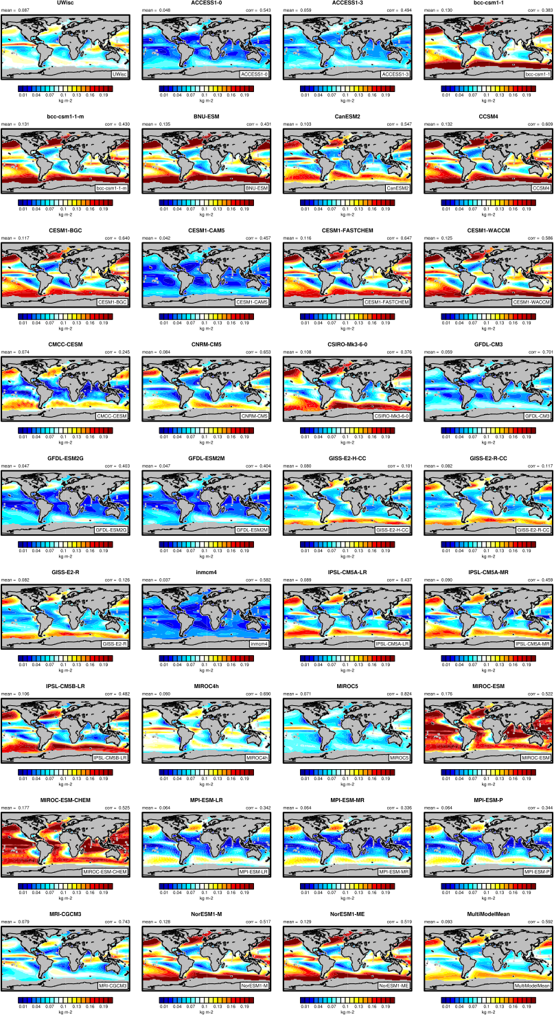
Fig. 139 The 20-yr average LWP (1986-2005) from the CMIP5 historical model runs and the multi-model mean in comparison with the UWisc satellite climatology (1988-2007) based on SSM/I, TMI, and AMSR-E (O’Dell et al. 2008). Produced with recipe_lauer13jclim.yml (diagnostic script clouds.ncl).#
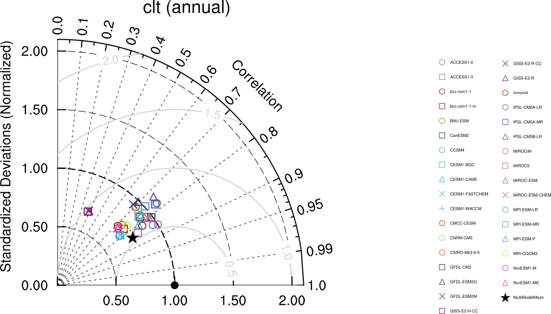
Fig. 140 Taylor diagram showing the 20-yr annual average performance of CMIP5 models for total cloud fraction as compared to MODIS satellite observations. Produced with recipe_lauer13jclim.yml (diagnostic script clouds_taylor.ncl).#
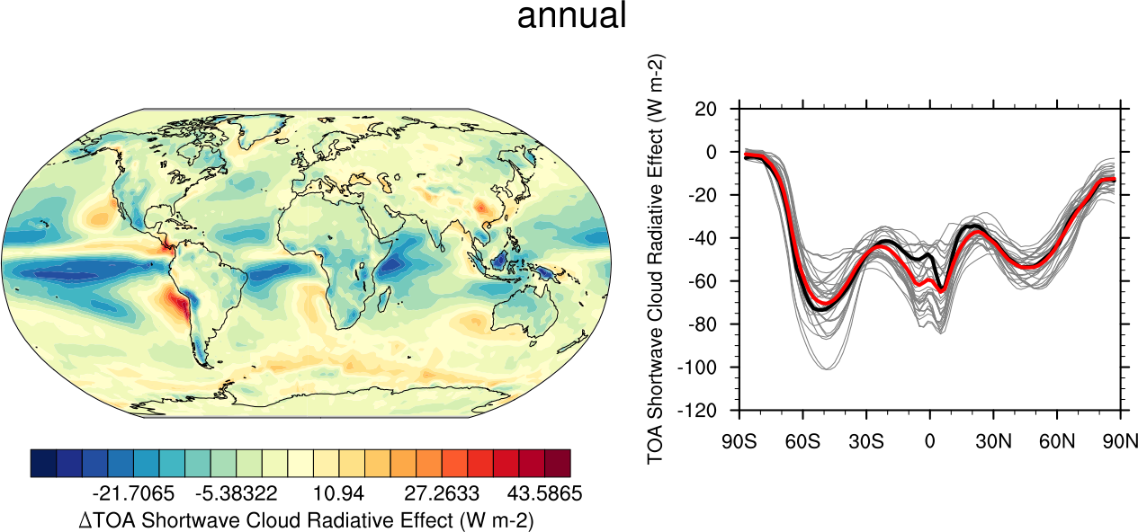

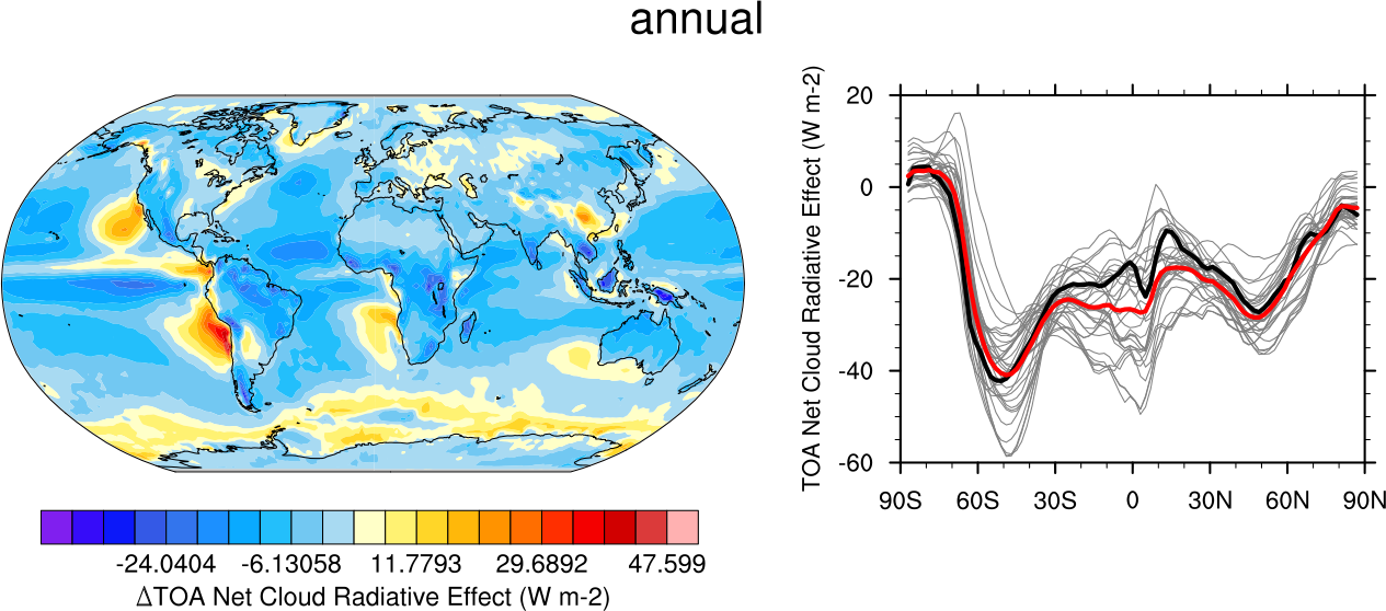
Fig. 141 20-year average (1986-2005) annual mean cloud radiative effects of CMIP5 models against the CERES-EBAF (2001–2012). Top row shows the shortwave effect; middle row the longwave effect, and bottom row the net effect. Multi-model mean biases against CERES-EBAF are shown on the left, whereas the right panels show zonal averages from CERES-EBAF (thick black), the individual CMIP5 models (thin gray lines) and the multi-model mean (thick red line). Similar to Figure 9.5 of Flato et al., 2013. Produced with recipe_clouds_ipcc.yml (diagnostic script clouds_ipcc.ncl).#
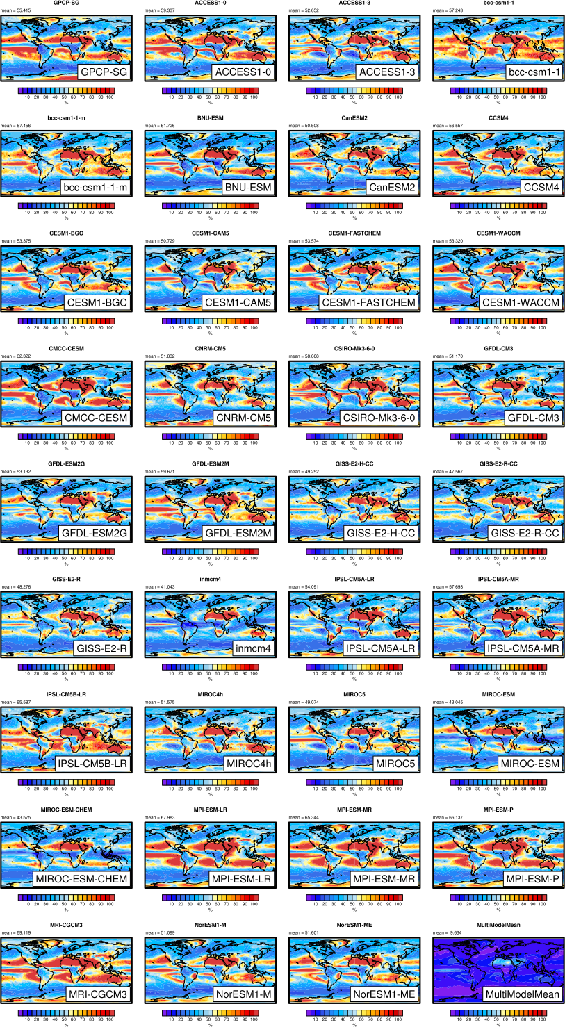
Fig. 142 Interannual variability of modeled and observed (GPCP) precipitation rates estimated as relative temporal standard deviation from 20 years (1986-2005) of data. The temporal standard deviations are calculated from monthly anomalies after subtracting the climatological mean seasonal cycle. Produced with recipe_lauer13jclim.yml (clouds_interannual.ncl).#
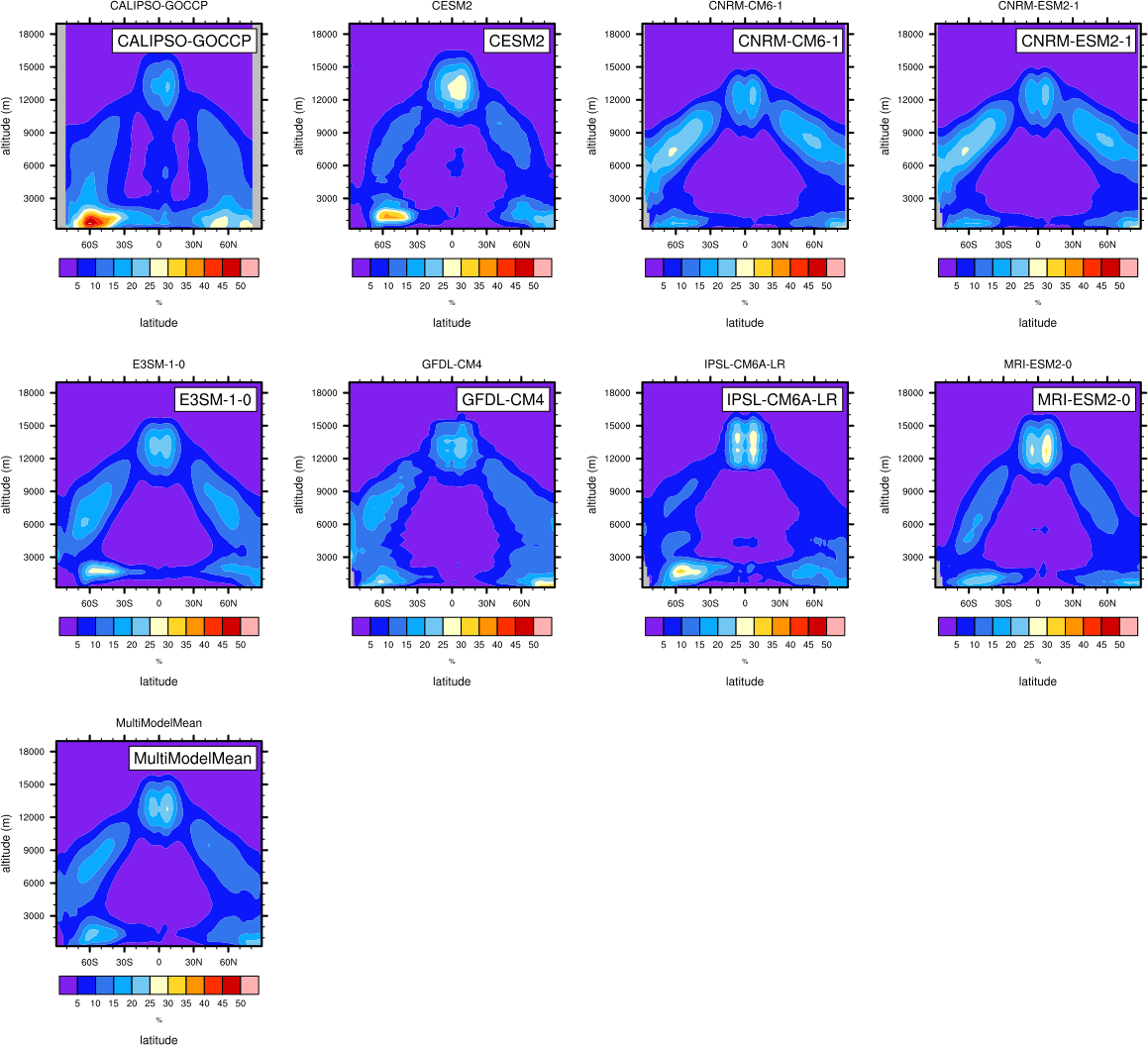
Fig. 143 Zonal mean of the multi-year annual mean cloud fraction as seen from CALIPSO from CMIP6 models in comparison to CALIPSO-GOCCP data. Produced with recipe_lauer22jclim_fig3-4_zonal.yml (diagnostic script clouds_zonal.ncl).#
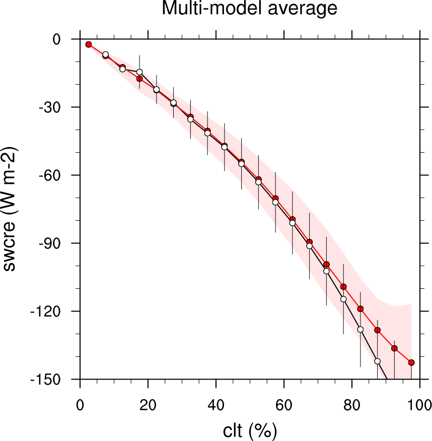
Fig. 144 Multi-year seasonal average (December-January-February) of cloud shortwave radiative effect (W m-2) vs. total cloud fraction (clt, %) averaged over the Southern Ocean defined as latitude belt 30°S-65°S (ocean grid cells only). Shown are the CMIP6 multi-model mean (red filled circles and lines) and observational estimates from ESACCI-CLOUD (black circles and lines). The red shaded areas represent the range between the 10th and 90th percentiles of the results from all individual models. Produced with recipe_lauer22jclim_fig9-11ab_scatter.yml (diagnostic script clouds_scatter.ncl).#
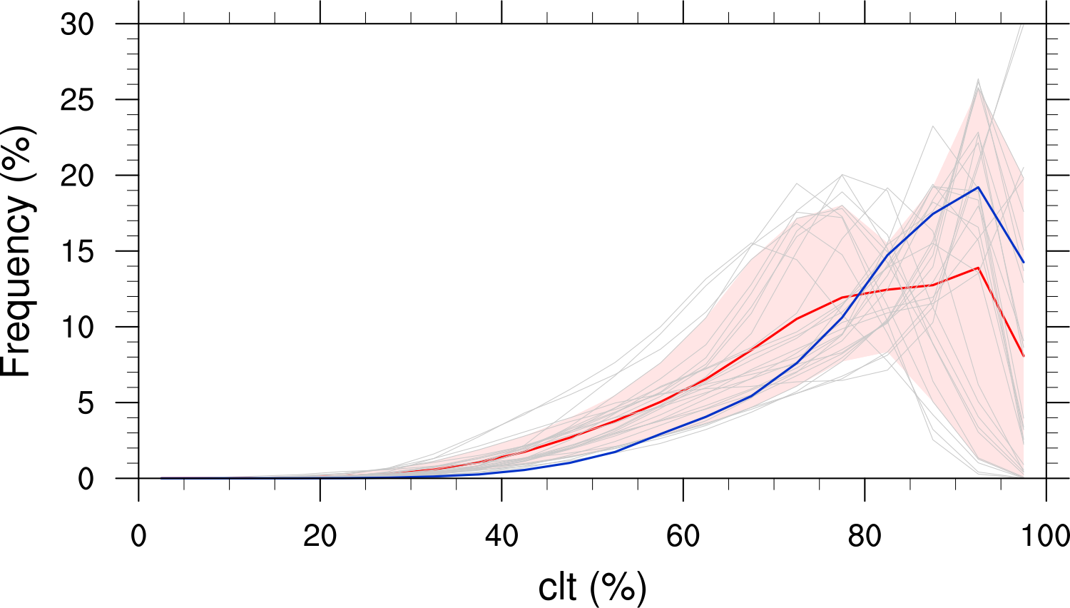
Fig. 145 Frequency distribution of monthly mean total cloud cover from CMIP6 models in comparison to ESACCI-CLOUD data. The red curve shows the multi-model average, the blue curve the ESACCI-CLOUD data and the thin gray lines the individual models. The red shading shows ±1 standard deviation of the inter-model spread. Produced with recipe_lauer22jclim_fig9-11c_pdf.yml (diagnostic script clouds_pdf.ncl).#
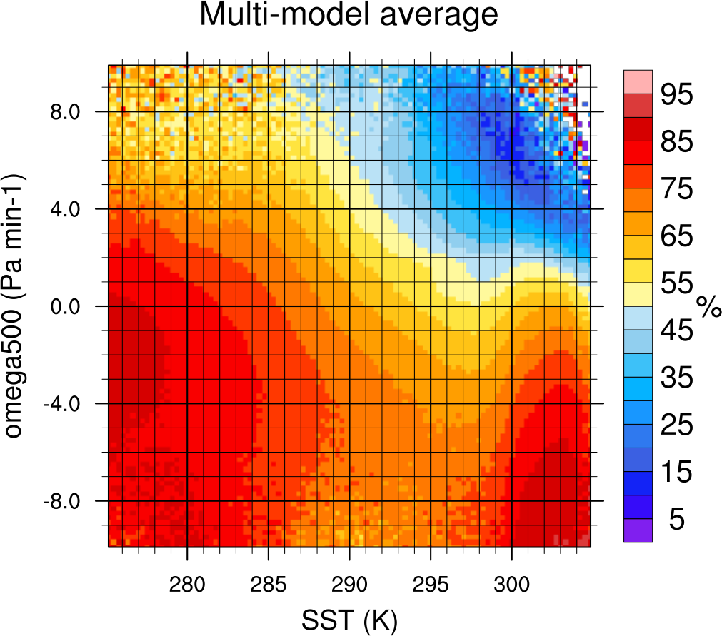
Fig. 146 2-dimensional distribution of average total cloud cover (clt) binned by sea surface temperature (SST, x-axis) and vertical velocity at 500 hPa (ω500, y-axis) averaged over 20 years and all grid cells over the ocean. Produced with recipe_lauer22jclim_fig8_dyn.yml (diagnostic script clouds_dyn_matrix.ncl).#