Equilibrium climate sensitivity
Overview
Equilibrium climate sensitivity is defined as the change in global mean temperature as a result of a doubling of the atmospheric CO2 concentration compared to pre-industrial times after the climate system has reached a new equilibrium. This recipe uses a regression method based on Gregory et al. (2004) to calculate it for several CMIP models.
Available recipes and diagnostics
Recipes are stored in recipes/
recipe_ecs.yml
Diagnostics are stored in diag_scripts/
climate_metrics/ecs.py
climate_metrics/create_barplot.py
climate_metrics/create_scatterplot.py
User settings in recipe
Preprocessor
area_statistics(operation: mean): Calculate global mean.
Script climate_metrics/ecs.py
calculate_mmm, bool, optional (default:True): Calculate multi-model mean ECS.complex_gregory_plot, bool, optional (default:False): Plot complex Gregory plot (also add response for firstsep_yearyears and last 150 -sep_yearyears, default:sep_year=20) ifTrue.output_attributes, dict, optional: Write additional attributes to netcdf files.read_external_file, str, optional: Read ECS and feedback parameters from external file. The path can be given relative to this diagnostic script or as absolute path.savefig_kwargs, dict, optional: Keyword arguments formatplotlib.pyplot.savefig().seaborn_settings, dict, optional: Options forseaborn.set()(affects all plots).sep_year, int, optional (default:20): Year to separate regressions of complex Gregory plot. Only effective ifcomplex_gregory_plotisTrue.x_lim, list of float, optional (default:[1.5, 6.0]): Plot limits for X axis of Gregory regression plot (T).y_lim, list of float, optional (default:[0.5, 3.5]): Plot limits for Y axis of Gregory regression plot (N).
Script climate_metrics/create_barplot.py
add_mean, str, optional: Add a bar representing the mean for each class.label_attribute, str, optional: Cube attribute which is used as label for different input files.order, list of str, optional: Specify the order of the different classes in the barplot by giving thelabel, makes most sense when combined withlabel_attribute.patterns, list of str, optional: Patterns to filter list of input data.savefig_kwargs, dict, optional: Keyword arguments formatplotlib.pyplot.savefig().seaborn_settings, dict, optional: Options forseaborn.set()(affects all plots).sort_ascending, bool, optional (default:False): Sort bars in ascending order.sort_descending, bool, optional (default:False): Sort bars in descending order.subplots_kwargs, dict, optional: Keyword arguments formatplotlib.pyplot.subplots().value_labels, bool, optional (default:False): Label bars with value of that bar.y_range, list of float, optional: Range for the Y axis of the plot.
Script climate_metrics/create_scatterplot.py
dataset_style, str, optional: Name of the style file (located inesmvaltool.diag_scripts.shared.plot.styles_python).pattern, str, optional: Pattern to filter list of input files.seaborn_settings, dict, optional: Options forseaborn.set()(affects all plots).y_range, list of float, optional: Range for the Y axis of the plot.
Variables
rlut (atmos, monthly, longitude, latitude, time)
rsdt (atmos, monthly, longitude, latitude, time)
rsut (atmos, monthly, longitude, latitude, time)
tas (atmos, monthly, longitude, latitude, time)
Observations and reformat scripts
None
References
Gregory, Jonathan M., et al. “A new method for diagnosing radiative forcing and climate sensitivity.” Geophysical research letters 31.3 (2004).
Example plots
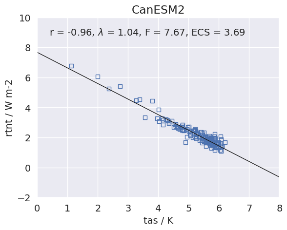
Fig. 106 Scatterplot between TOA radiance and global mean surface temperature anomaly for 150 years of the abrupt 4x CO2 experiment including linear regression to calculate ECS for CanESM2 (CMIP5).