Climate model Weighting by Independence and Performance (ClimWIP)
Overview
Projections of future climate change are often based on multi-model ensembles of global climate models such as CMIP6. To condense the information from these models they are often combined into probabilistic estimates such as mean and a related uncertainty range (such as the standard deviation). However, not all models in a given multi-model ensemble are always equally ‘fit for purpose’ and it can make sense to weight models based on their ability to simulate observed quantities related to the target. In addition, multi-model ensembles, such as CMIP can contain several models based on a very similar code-base (sharing of components, only differences in resolution etc.) leading to complex inter-dependencies between the models. Adjusting for this by weighting models according to their independence helps to adjust for this.
This recipe implements the Climate model Weighting by Independence and Performance
(ClimWIP) method. It is based on work by Knutti et al. (2017),
Lorenz et al. (2018),
Brunner et al. (2019),
Merrifield et al. (2020),
Brunner et al. (2020). Weights are
calculated based on historical model performance in several metrics (which can be
defined by the performance_contributions parameter) as well as by their independence
to all the other models in the ensemble based on their output fields in several metrics
(which can be defined by the independence_contributions parameter). These weights
can be used in subsequent evaluation scripts (some of which are implemented as part of
this diagnostic).
Note: this recipe is still being developed! A more comprehensive (yet older) implementation can be found on GitHub: https://github.com/lukasbrunner/ClimWIP
Using shapefiles for cutting scientific regions
To use shapefiles for selecting SREX or AR6 regions by name it is necessary to download them, e.g., from the sources below and reference the file using the shapefile parameter. This can either be a absolute or a relative path. In the example recipes they are stored in a subfolder shapefiles in the auxiliary_data_dir (with is specified in the config-user.yml).
SREX regions (AR5 reference regions): http://www.ipcc-data.org/guidelines/pages/ar5_regions.html
AR6 reference regions: https://github.com/SantanderMetGroup/ATLAS/tree/v1.6/reference-regions
Available recipes and diagnostics
Recipes are stored in esmvaltool/recipes/
recipe_climwip_test_basic.yml: Basic sample recipe using only a few models
recipe_climwip_test_performance_sigma.yml: Advanced sample recipe for testing the perfect model test in particular
recipe_climwip_brunner2019_med.yml: Slightly modified results for one region from Brunner et al. (2019) (to change regions see below)
recipe_climwip_brunner2020esd.yml: Slightly modified results for Brunner et al. (2020)
Diagnostics are stored in esmvaltool/diag_scripts/weighting/climwip/
main.py: Compute weights for each input dataset
calibrate_sigmas.py: Compute the sigma values on the fly
core_functions.py: A collection of core functions used by the scripts
io_functions.py: A collection of input/output functions used by the scripts
Plot scripts are stored in esmvaltool/diag_scripts/weighting/
weighted_temperature_graph.py: Show the difference between weighted and non-weighted temperature anomalies as time series.
weighted_temperature_map.py: Show the difference between weighted and non-weighted temperature anomalies on a map.
plot_utilities.py: A collection of functions used by the plot scripts.
User settings in recipe
Script
main.py
- Required settings for script
performance_sigmaxorcalibrate_performance_sigma: Ifperformance_contributionsis given exactly one of the two has to be given. Otherwise they can be skipped or not set.
performance_sigma: float setting the shape parameter for the performance weights calculation (determined offline).
calibrate_performance_sigma: dictionary setting the performance sigma calibration. Has to contain at least the key-value pair specifyingtarget:variable_group. Optional parameters for adjusting the calibration are not yet implemented. Warning: It is highly recommended to visually inspect the graphical output of the calibration to check if everything worked as intended. In case the calibration fails, the best performance sigma will still be indicated in the figure (see example Fig. 73 below) but not automatically picked - the user can decide to use it anyway by setting it in the recipe (not recommenced).
independence_sigma: float setting the shape parameter for the independence weights calculation (determined offline). Can be skipped or not set ifindependence_contributionsis skipped or not set. A on-the-fly calculation of the independence sigma is not yet implemented
performance_contributions: dictionary where the keys represent the variable groups to be included in the performance calculation. The values give the relative contribution of each group, with 0 being equivalent to not including the group. Can be skipped or not set then weights will be based purely on model independence (this is mutually exclusive withindependence_contributionsbeing skipped or not set).
independence_contributions: dictionary where the keys represent the variable groups to be included in the independence calculation. The values give the relative contribution of each group, with 0 being equivalent to not including the group. If skipped or not set weights will be based purely on model performance (this is mutually exclusive withperformance_contributionsbeing skipped or not set).
combine_ensemble_members: set to true if ensemble members of the same model should be combined during the processing (leads to identical weights for all ensemble members of the same model). Recommended if running with many (>10) ensemble members per model. If set to false, the model independence weighting will still (partly) account for the (very high) dependence between members of the same model. The success of this will depend on the case and the selected parameters. See Merrifield et al. (2020) for an in-depth discussion.
obs_data: list of project names to specify which are the observational data. The rest is assumed to be model data.Required settings for variables * This script takes multiple variables as input as long as they’re available for all models *
start_year: provide the period for which to compute performance and independence. *end_year: provide the period for which to compute performance and independence. *mip: typically Amon *preprocessor: e.g., climatological_mean *additional_datasets: this should be*obs_dataand is only needed for variables used inperformance_contributions.
- Required settings for preprocessor
Different combinations of preprocessor functions can be used, but the end result should always be aggregated over the time dimension, i.e. the input for the diagnostic script should be 2d (lat/lon).
- Optional settings for preprocessor
extract_regionorextract_shapecan be used to crop the input data.
extract_seasoncan be used to focus on a single season.different climate statistics can be used to calculate mean, (detrended) std_dev, or trend.
Script
weighted_temperature_graph.py
- Required settings for script
ancestors: must include weights from previous diagnostic
weights: the filename of the weights: ‘weights.nc’
settings: a list of plot settings:start_year(integer),end_year(integer),central_estimate(‘mean’ or integer between 0 and 100 giving the percentile),lower_bound(integer between 0 and 100),upper_bound(integer between 0 and 100)- Required settings for variables
This script only takes temperature (tas) as input
start_year: provide the period for which to plot a temperature change graph.
end_year: provide the period for which to plot a temperature change graph.
mip: typically Amon
preprocessor: temperature_anomalies- Required settings for preprocessor
Different combinations of preprocessor functions can be used, but the end result should always be aggregated over the latitude and longitude dimensions, i.e. the input for the diagnostic script should be 1d (time).
- Optional settings for preprocessor
Can be a global mean or focus on a point, region or shape
Anomalies can be calculated with respect to a custom reference period
Monthly, annual or seasonal average/extraction can be used
Script
weighted_temperature_map.py- Required settings for script
ancestors: must include weights from previous diagnosticweights: the filename of the weights: ‘weights_combined.nc’
- Optional settings for script
model_aggregation: how to aggregate the models: mean (default), median, integer between 0 and 100 representing a percentilexticks: positions to draw xticks atyticks: positions to draw yticks at
- Required settings for variables
This script takes temperature (tas) as input
start_year: provide the period for which to plot a temperature change graph.end_year: provide the period for which to plot a temperature change graph.mip: typically Amonpreprocessor: temperature_anomalies
- Optional settings for variables
A second variable is optional: temperature reference (tas_reference). If given, maps of temperature change to the reference are drawn, otherwise absolute temperatures are drawn.
tas_reference takes the same fields as tas
Updating the Brunner et al. (2019) recipe for new regions
recipe_climwip_brunner2019_med.yml demonstrates a very similar setup to Brunner et al. (2019)
but only for one region (the Mediterranean). To calculated weights for other regions the recipe needs to be updated in two places:
extract_shape:
   shapefile: shapefiles/srex.shp
   decomposed: True
   method: contains
   crop: true
   ids:
     - 'South Europe/Mediterranean [MED:13]'
The ids field takes any valid SREX region
key or any valid AR6 region key
(depending on the shapefile). Note that this needs to be the full string here (not the abbreviation).
The sigma parameters need to be set according to the selected region. The sigma values for the regions used in Brunner et al. (2019) can be found in table 1 of the paper.
performance_sigma: 0.546
independence_sigma: 0.643
Warning: if a new region is used the sigma values should be recalculated! This can be done by commenting out the sigma values (lines above) and commenting in the blocks defining the target of the weighting:
CLIM_future:
   short_name: tas
   start_year: 2081
   end_year: 2100
   mip: Amon
   preprocessor: region_mean
as well as
calibrate_performance_sigma:
   target: CLIM_future
In this case ClimWIP will attempt to perform an on-the-fly perfect model test to estimate the lowest performance sigma (strongest weighting) which does not lead to overconfident weighting. Important: the user should always check the test output for unusual behaviour. For most cases the performance sigma should lie around 0.5. In cases where the perfect model test fails (no appropriate performance sigma can be found) the test will still produce graphical output before raising a ValueError. The user can then decide to manually set the performance sigma to the most appropriate value (based on the output) - this is not recommended and should only be done with care! The perfect model test failing can be a hint for one of the following: (1) not enough models in the ensemble for a robust distribution (normally >20 models should be used) or (2) the performance metrics used are not relevant for the target.
An on-the-fly calibration for the independence sigma is not yet implemented. For most cases we recommend to use the same setup as in Brunner et al. (2020) or Merrifield et al. (2020) (global or hemispherical temperature and sea level pressure climatologies as metrics and independence sigma values between 0.2 and 0.5).
Warning: if a new region or target is used the provided metrics to establish the weights might no longer be appropriate. Using unrelated metrics with no correlation and/or physical relation to the target will reduce the skill of the weighting and ultimately render it useless! In such cases the perfect model test might fail. This means the performance metrics should be updated.
Brunner et al. (2020) recipe and example independence weighting
recipe_climwip_brunner2020esd.yml implements the weighting used in Brunner et al. (2020). Compared to the paper there are minor differences due to two models which had to be excluded due to errors in the ESMValTool pre-processor: CAMS-CSM1-0 and MPI-ESM1-2-HR (r2) as well as the use of only one observational dataset (ERA5).
The recipe uses an additional step between pre-processor and weight calculation to calculate anomalies relative to the global mean (e.g., tas_ANOM = tas_CLIM - global_mean(tas_CLIM)). This means we do not use the absolute temperatures of a model as performance criterion but rather the horizontal temperature distribution (see Brunner et al. 2020 for a discussion).
This recipe also implements a somewhat general independence weighting for CMIP6. In contrast to model performance (which should be case specific) model independence can largely be seen as only dependet on the multi-model ensemble in use but not the target variable or region. This means that the configuration used should be valid for similar subsets of CMIP6 as used in this recipe:
combine_ensemble_members: true
independence_sigma: 0.54
independence_contributions:
    tas_CLIM_i: 1
    psl_CLIM_i: 1
Note that this approach weights ensemble members of the same model with a 1/N independence scaling (combine_ensemble_members: true) as well as different models with an output-based independence weighting. Different approaches to handle ensemble members are discussed in Merrifield et al. (2020). Note that, unlike for performance, climatologies are used for independence (i.e., the global mean is not removed for independence). Warning: Using only the independence weighting without any performance weighting might not always lead to meaningful results! The independence weighting is based on model output, which means that if a model is very different from all other models as well as the observations it will get a very high independence weight (and also total weight in absence of any performance weighting). This might not reflect the actual independence. It is therefore recommended to use weights based on both independence and performance for most cases.
Variables
pr (atmos, monthly mean, longitude latitude time)
tas (atmos, monthly mean, longitude latitude time)
psl (atmos, monthly mean, longitude latitude time)
rsus, rsds, rlus, rlds, rsns, rlns (atmos, monthly mean, longitude latitude time)
more variables can be added if available for all datasets.
Observations and reformat scripts
Observation data is defined in a separate section in the recipe and may include multiple datasets.
References
Brunner et al. (2020), Earth Syst. Dynam., 11, 995-1012
Merrifield et al. (2020), Earth Syst. Dynam., 11, 807-834
Brunner et al. (2019), Environ. Res. Lett., 14, 124010
Lorenz et al. (2018), J. Geophys. Res.: Atmos., 9, 4509-4526
Knutti et al. (2017), Geophys. Res. Lett., 44, 1909-1918
Example plots
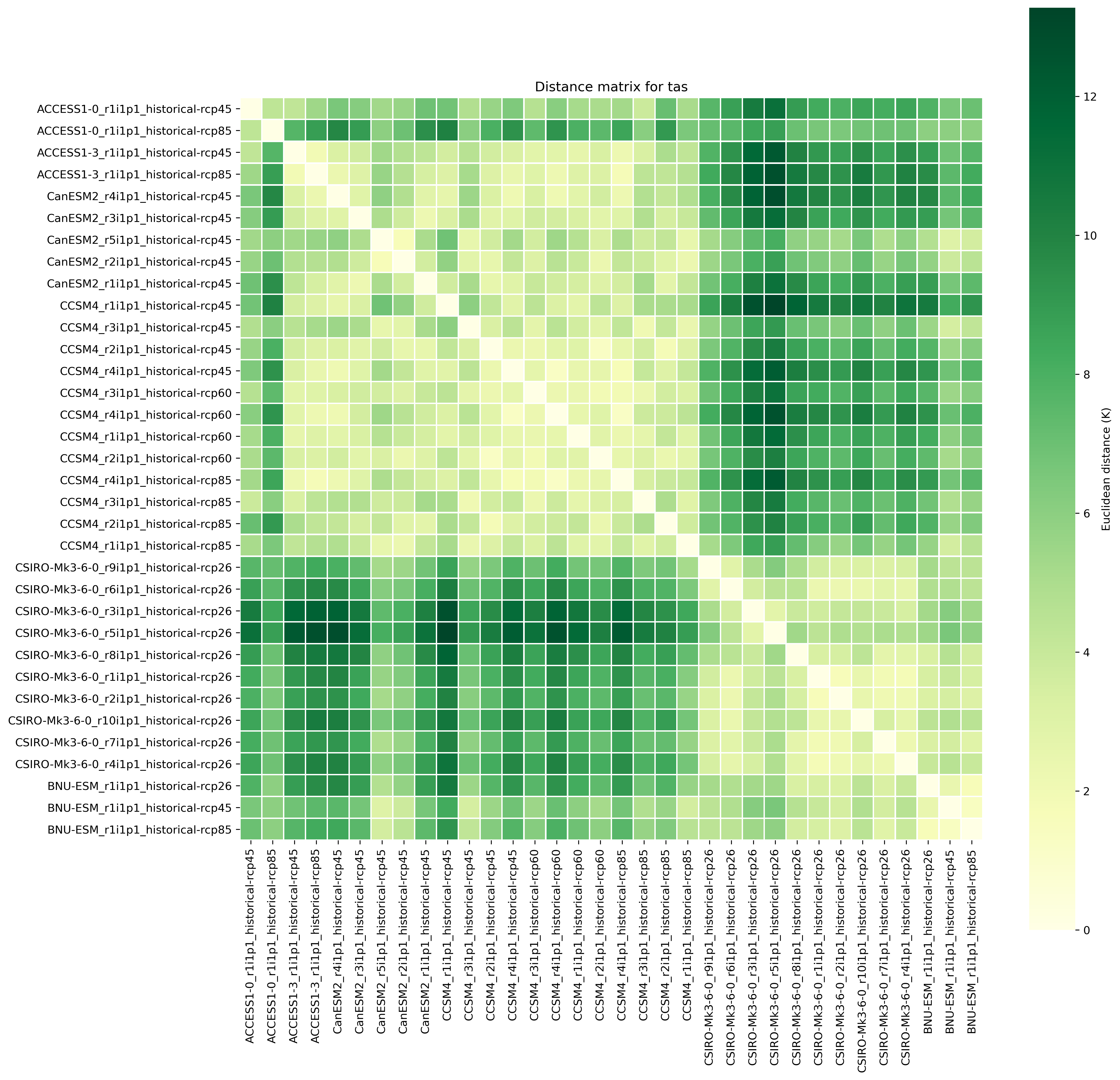
Fig. 69 Distance matrix for temperature, providing the independence metric.
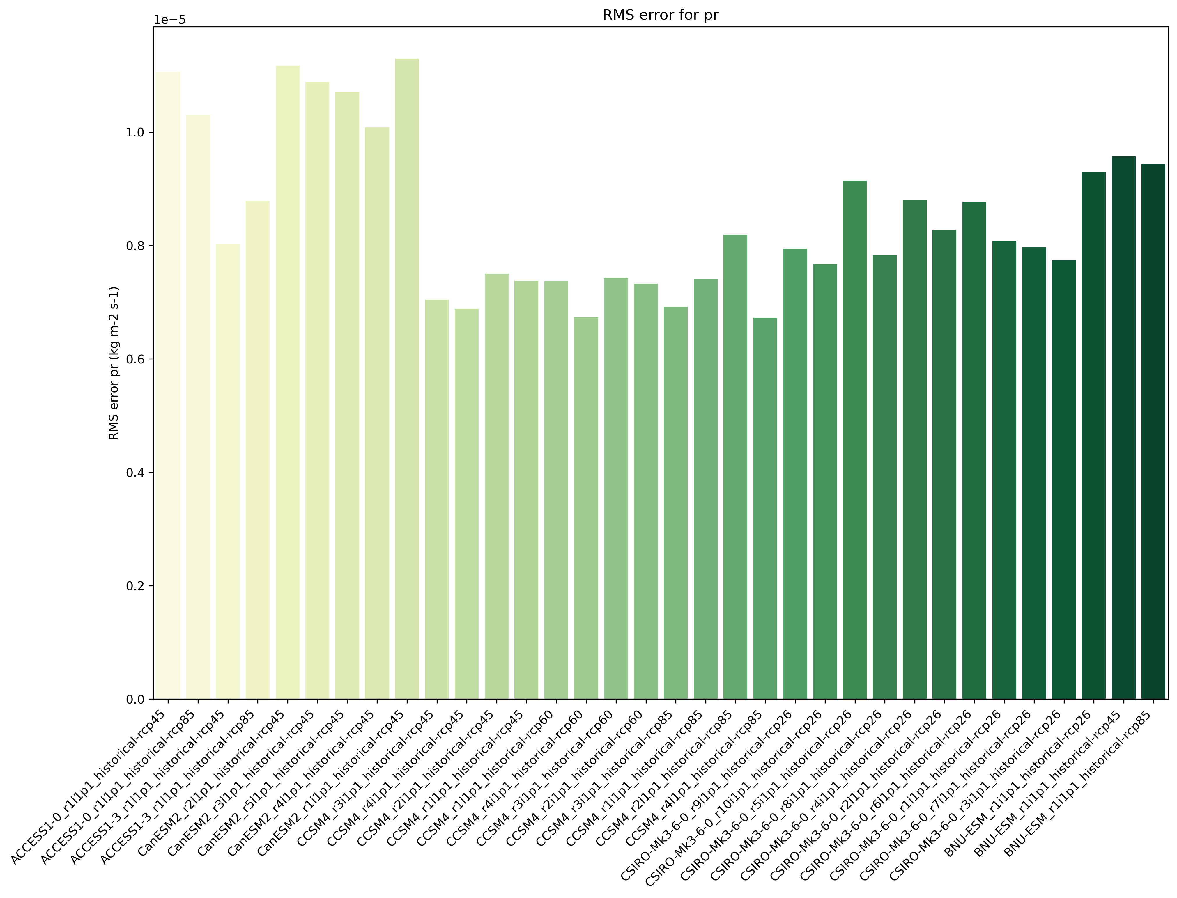
Fig. 70 Distance of preciptation relative to observations, providing the performance metric.
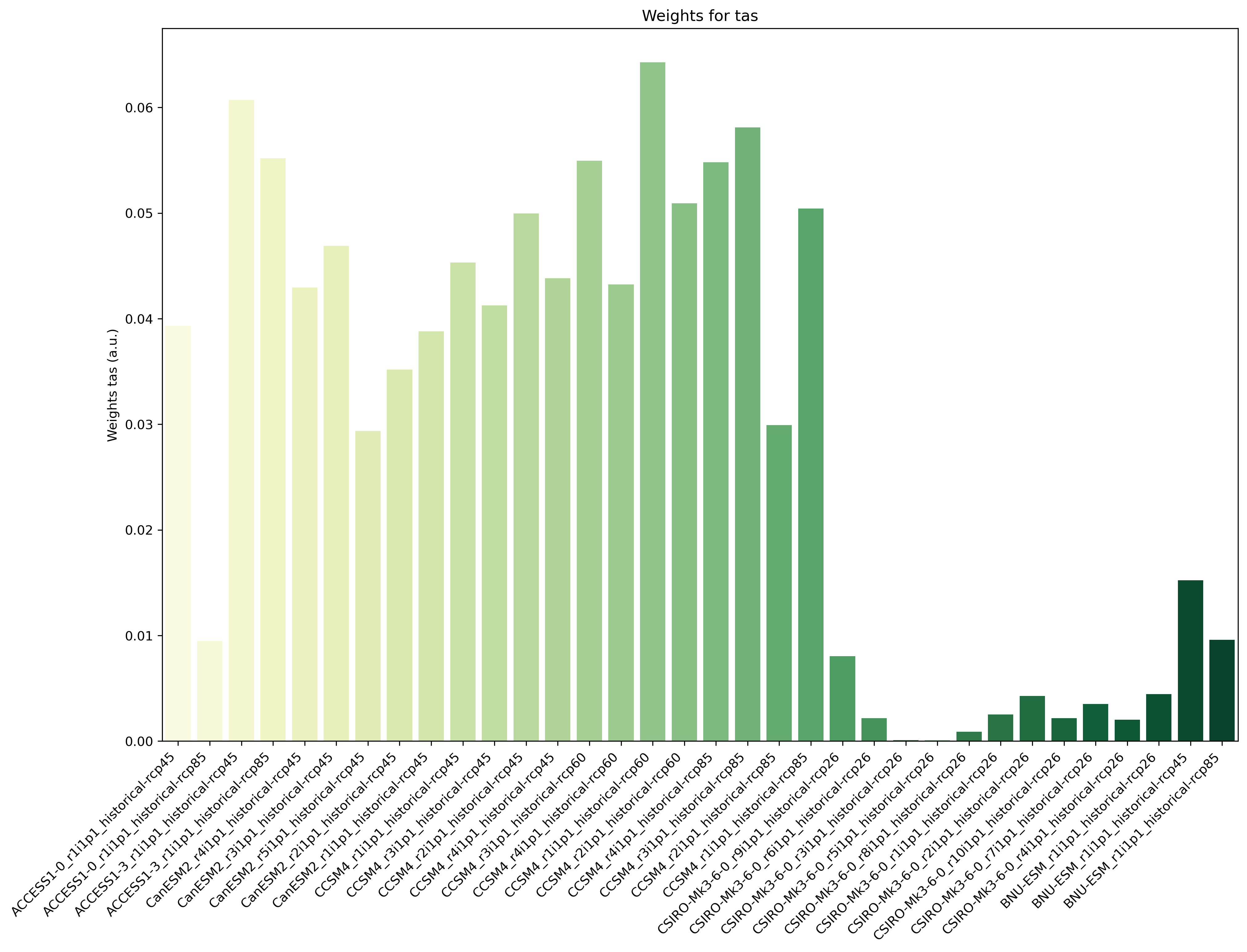
Fig. 71 Weights determined by combining independence and performance metrics for tas.
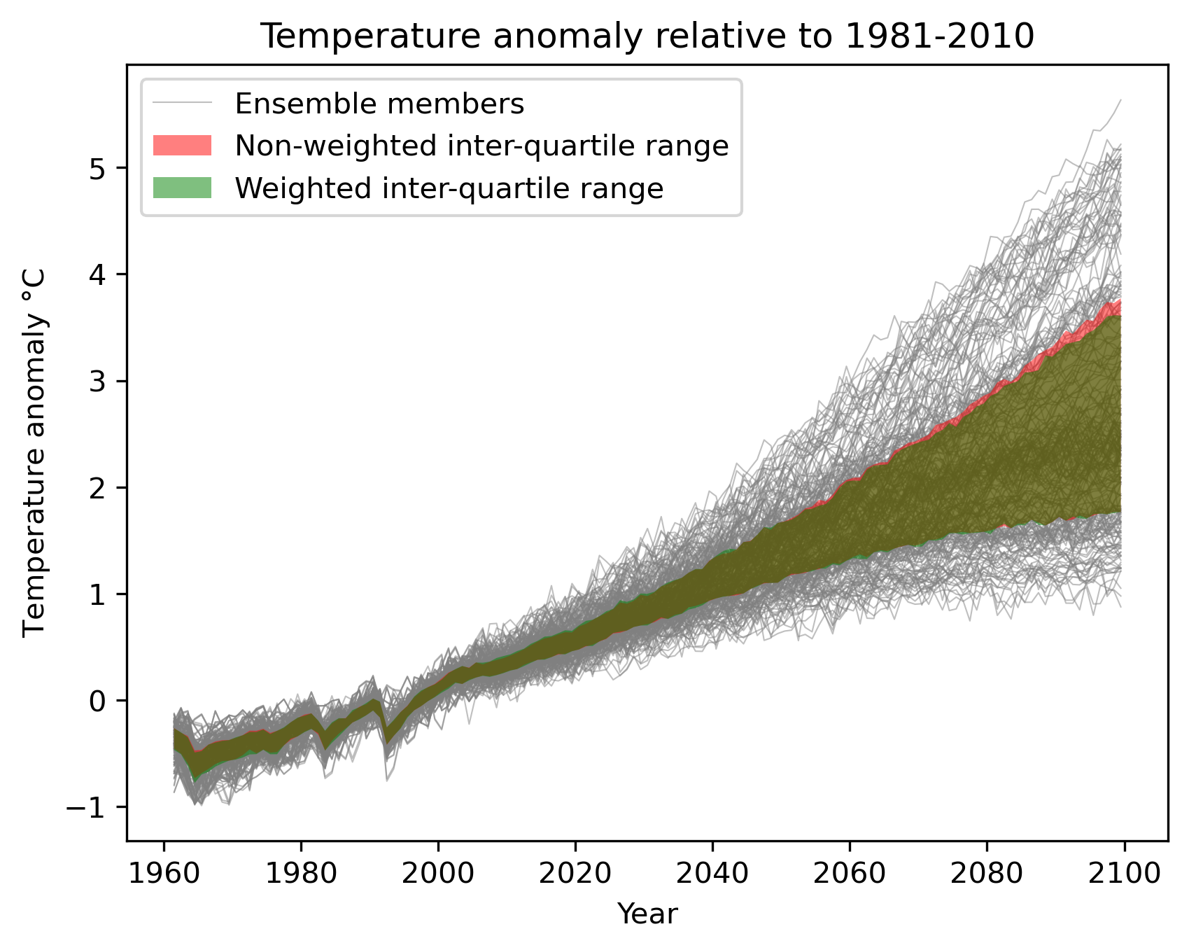
Fig. 72 Interquartile range of temperature anomalies relative to 1981-2010, weighted versus non-weighted.
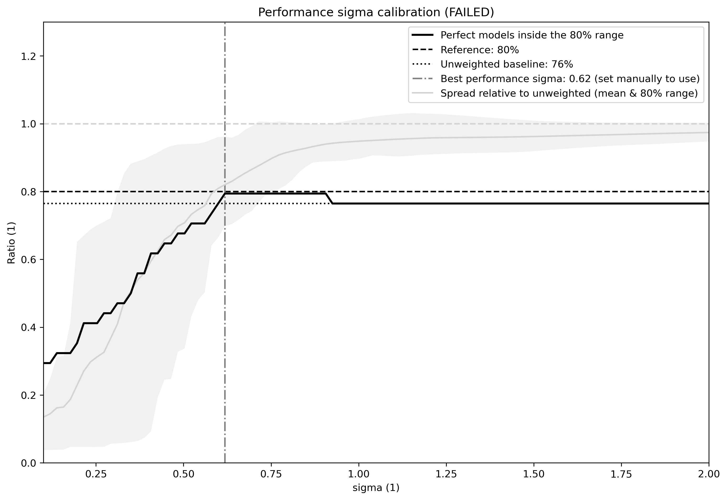
Fig. 73 Performance sigma calibration: The thick black line gives the reliability (c.f., weather forecast verification) which should reach at least 80%. The thick grey line gives the mean change in spread between the unweighted and weighted 80% ranges as an indication of the weighting strength (if it reaches 1, the weighting has no effect on uncertainty). The smallest sigma (i.e., strongest weighting) which is not overconfident (reliability >= 80%) is selected. If the test fails (like in this example) the smallest sigma which comes closest to 80% will be indicated in the legend (but NOT automatically selected).
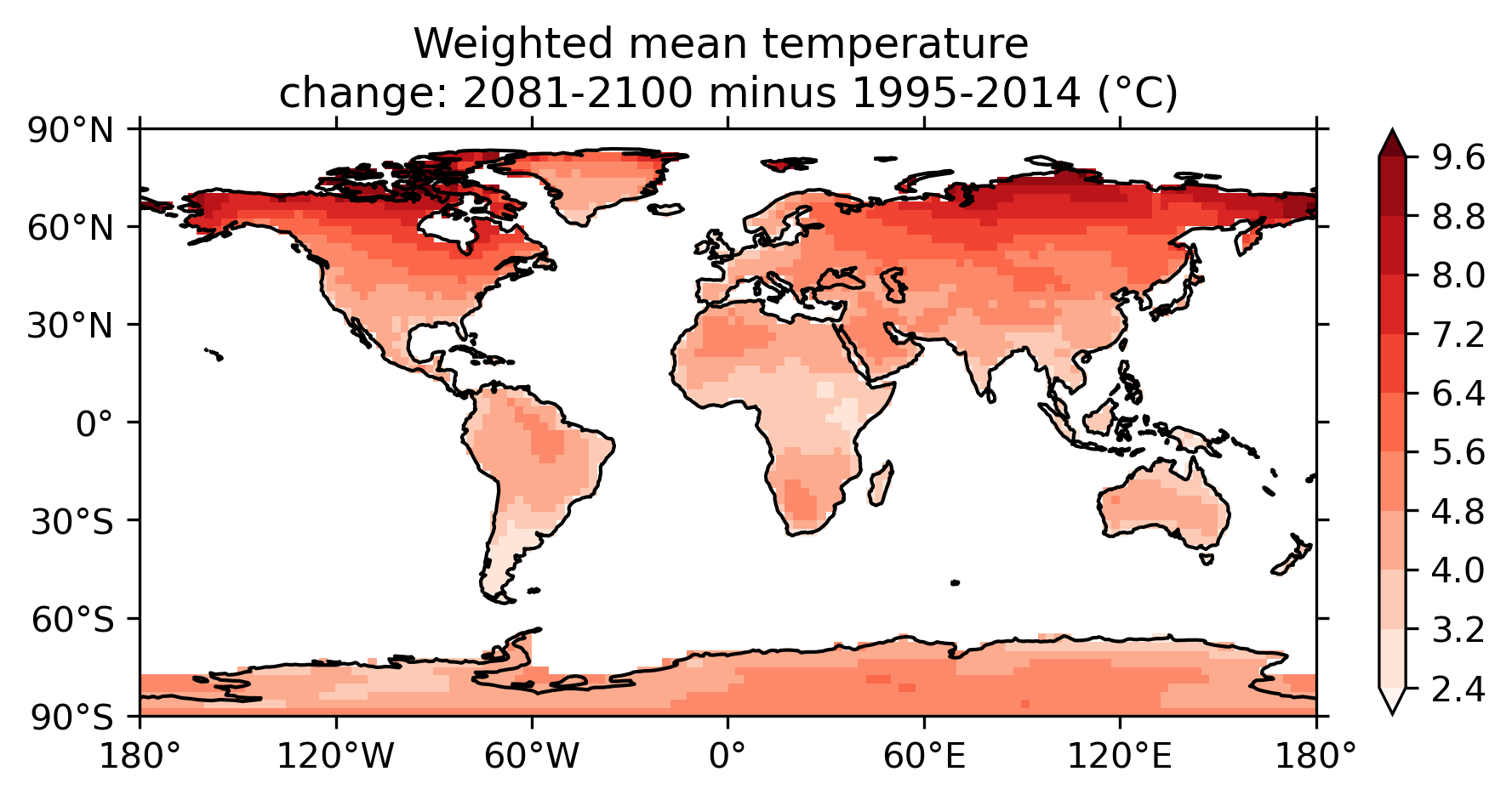
Fig. 74 Map of weighted mean temperature change 2081-2100 relative to 1995-2014