Evaluate water vapor short wave radiance absorption schemes of ESMs with the observations.
Overview
The recipe reproduces figures from DeAngelis et al. (2015): Figure 1b to 4 from the main part as well as extended data figure 1 and 2. This paper compares models with different schemes for water vapor short wave radiance absorption with the observations. Schemes using pseudo-k-distributions with more than 20 exponential terms show the best results.
Available recipes and diagnostics
Recipes are stored in recipes/
recipe_deangelis15nat.yml
Diagnostics are stored in diag_scripts/
deangelis15nat/deangelisf1b.py
deangelis15nat/deangelisf2ext.py
deangelis15nat/deangelisf3f4.py
User settings in recipe
The recipe can be run with different CMIP5 and CMIP6 models. deangelisf1b.py: Several flux variables (W m-2) and up to 6 different model exeriements can be handeled. Each variable needs to be given for each model experiment. The same experiments must be given for all models. In DeAngelis et al. (2015) 150 year means are used but the recipe can handle any duration.
deangelisf2ext.py:
deangelisf3f4.py: For each model, two experiments must be given: a pre industrial control run, and a scenario with 4 times CO2. Possibly, 150 years should be given, but shorter time series work as well.
Variables
deangelisf1b.py: Tested for:
rsnst (atmos, monthly, longitude, latitude, time)
rlnst (atmos, monthly, longitude, latitude, time)
lvp (atmos, monthly, longitude, latitude, time)
hfss (atmos, monthly, longitude, latitude, time)
any flux variable (W m-2) should be possible.
deangelisf2ext.py:
rsnst (atmos, monthly, longitude, latitude, time)
rlnst (atmos, monthly, longitude, latitude, time)
rsnstcs (atmos, monthly, longitude, latitude, time)
rlnstcs (atmos, monthly, longitude, latitude, time)
lvp (atmos, monthly, longitude, latitude, time)
hfss (atmos, monthly, longitude, latitude, time)
tas (atmos, monthly, longitude, latitude, time)
deangelisf3f4.py: * rsnstcs (atmos, monthly, longitude, latitude, time) * rsnstcsnorm (atmos, monthly, longitude, latitude, time) * prw (atmos, monthly, longitude, latitude, time) * tas (atmos, monthly, longitude, latitude, time)
Observations and reformat scripts
deangelisf1b.py: * None
deangelisf2ext.py: * None
deangelisf3f4.py:
- rsnstcs:
CERES-EBAF
- prw
ERA-Interim, SSMI
References
DeAngelis, A. M., Qu, X., Zelinka, M. D., and Hall, A.: An observational radiative constraint on hydrologic cycle intensification, Nature, 528, 249, 2015.
Example plots
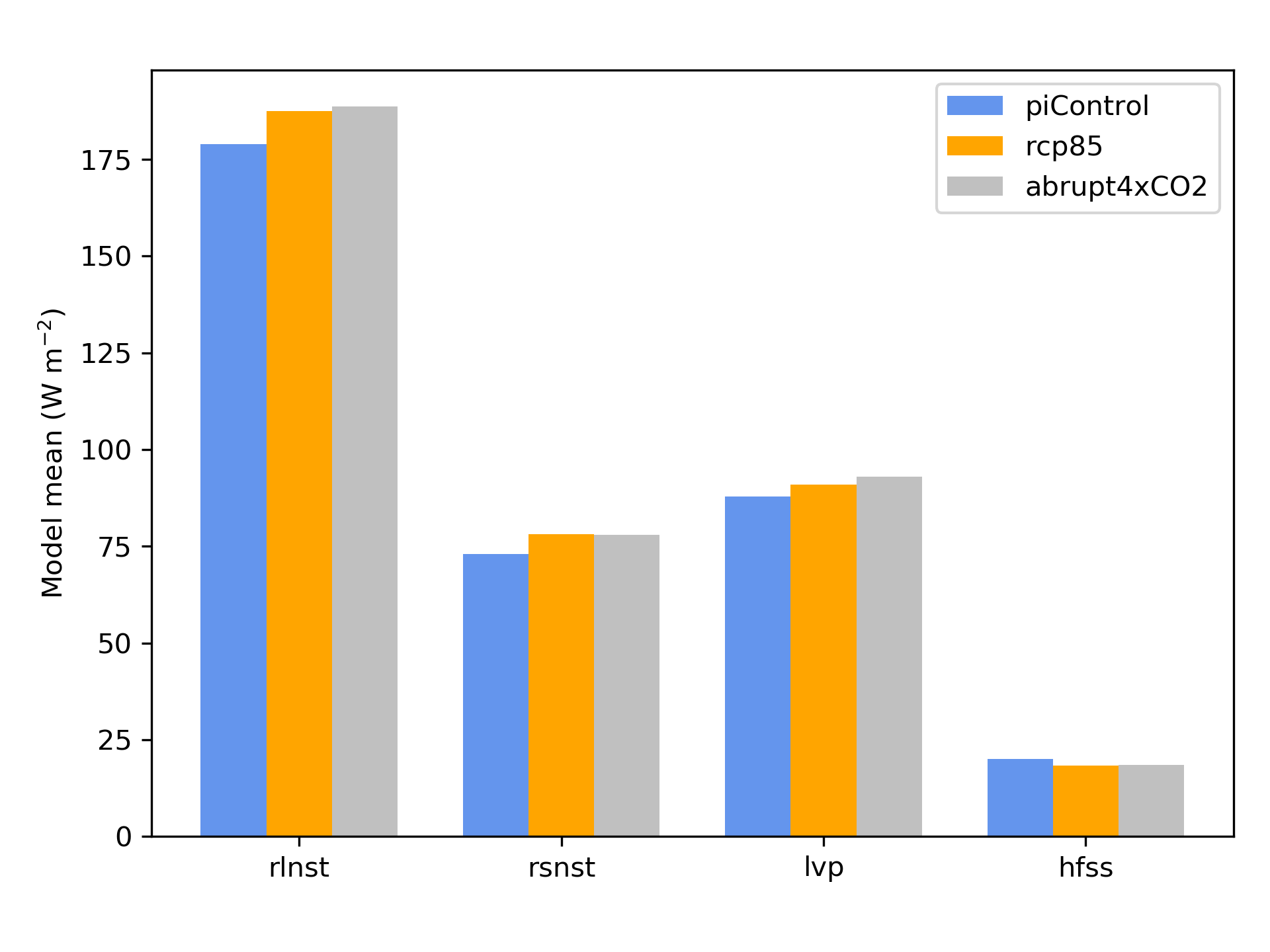
Fig. 15 Global average multi-model mean comparing different model experiments for the sum of upward long wave flux at TOA and net downward long wave flux at the surface (rlnst), heating from short wave absorption (rsnst), latent heat release from precipitation (lvp), and sensible heat flux (hfss). The panel shows three model experiments, namely the pre-industrial control simulation averaged over 150 years (blue), the RCP8.5 scenario averaged over 2091-2100 (orange) and the abrupt quadrupled CO2 scenario averaged over the years 141-150 after CO2 quadrupling in all models except CNRM-CM5-2 and IPSL-CM5A-MR, where the average is calculated over the years 131-140 (gray). The figure shows that energy sources and sinks readjust in reply to an increase in greenhouse gases, leading to a decrease in the sensible heat flux and an increase in the other fluxes.
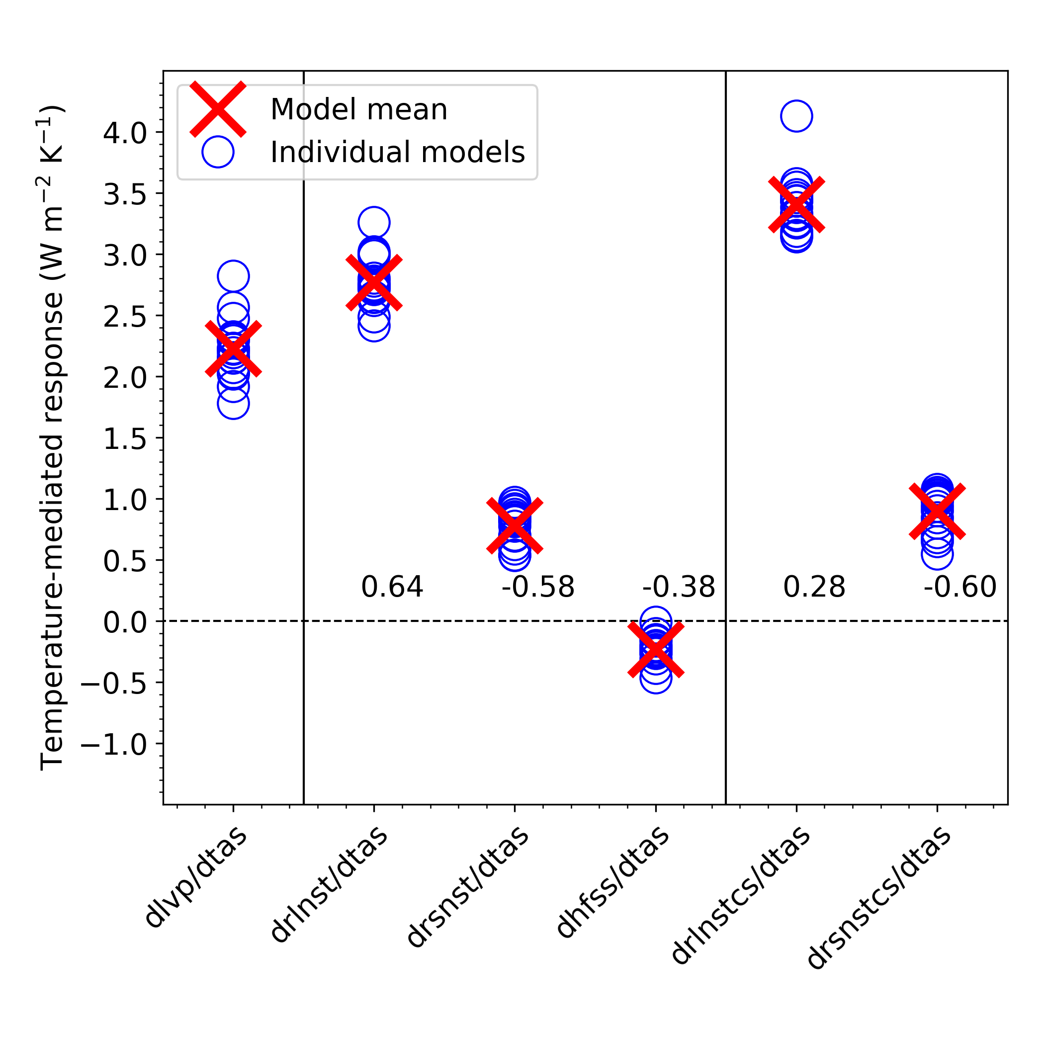
Fig. 16 The temperature-mediated response of each atmospheric energy budget term for each model as blue circles and the model mean as a red cross. The numbers above the abscissa are the cross-model correlations between dlvp/dtas and each other temperature-mediated response.’
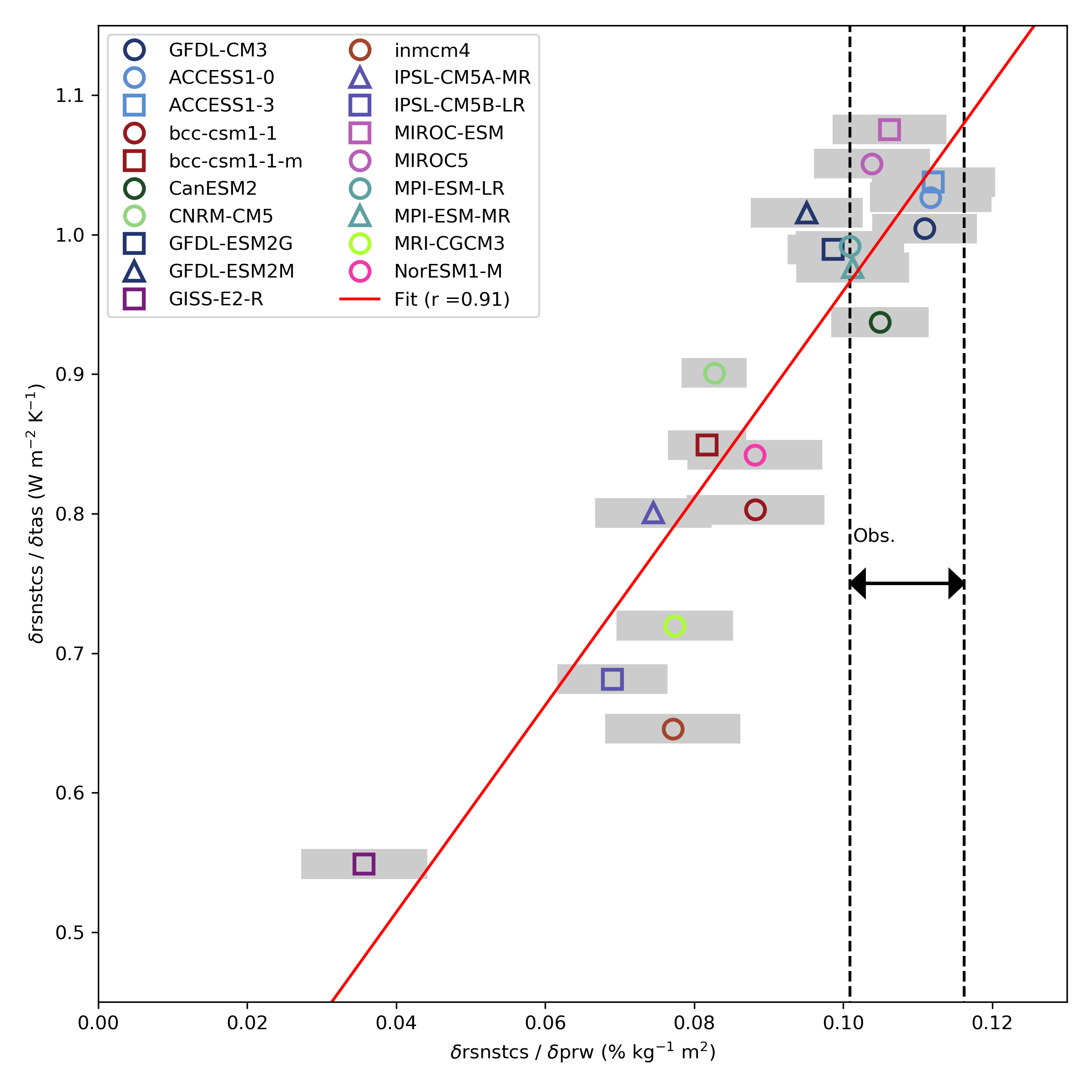
Fig. 17 Scatter plot and regression line the between the ratio of the change of net short wave radiation (rsnst) and the change of the Water Vapor Path (prw) against the ratio of the change of netshort wave radiation for clear skye (rsnstcs) and the the change of surface temperature (tas). The width of horizontal shading for models and the vertical dashed lines for observations (Obs.) represent statistical uncertainties of the ratio, as the 95% confidence interval (CI) of the regression slope to the rsnst versus prw curve. For the observations the minimum of the lower bounds of all CIs to the maximum of the upper bounds of all CIs is shown.