Clouds
Overview
The recipe recipe_lauer13jclim.yml computes the climatology and interannual variability of climate relevant cloud variables such as cloud radiative forcing (CRE), liquid water path (lwp), cloud amount (clt), and total precipitation (pr) reproducing some of the evaluation results of Lauer and Hamilton (2013). The recipe includes a comparison of the geographical distribution of multi-year average cloud parameters from individual models and the multi-model mean with satellite observations. Taylor diagrams are generated that show the multi-year annual or seasonal average performance of individual models and the multi-model mean in reproducing satellite observations. The diagnostic also facilitates the assessment of the bias of the multi-model mean and zonal averages of individual models compared with satellite observations. Interannual variability is estimated as the relative temporal standard deviation from multi-year timeseries of data with the temporal standard deviations calculated from monthly anomalies after subtracting the climatological mean seasonal cycle.
Available recipes and diagnostics
Recipes are stored in recipes/
recipe_lauer13jclim.yml
Diagnostics are stored in diag_scripts/clouds/
clouds.ncl: global maps of (multi-year) annual means including multi-model mean
clouds_bias.ncl: global maps of the multi-model mean and the multi-model mean bias
clouds_interannual: global maps of the interannual variability
clouds_isccp: global maps of multi-model mean minus observations + zonal averages of individual models, multi-model mean and observations
clouds_taylor.ncl: taylor diagrams
User settings in recipe
Script clouds.ncl
Required settings (scripts)
none
Optional settings (scripts)
embracesetup: true = 2 plots per line, false = 4 plots per line (default)
explicit_cn_levels: explicit contour levels (array)
extralegend: plot legend(s) to extra file(s)
filename_add: optionally add this string to plot filesnames
panel_labels: label individual panels (true, false)
PanelTop: manual override for “@gnsPanelTop” used by panel plot(s)
projection: map projection for plotting (default = “CylindricalEquidistant”)
showdiff: calculate and plot differences model - reference (default = false)
rel_diff: if showdiff = true, then plot relative differences (%) (default = False)
ref_diff_min: lower cutoff value in case of calculating relative differences (in units of input variable)
region: show only selected geographic region given as latmin, latmax, lonmin, lonmax
timemean: time averaging - “seasonal” = DJF, MAM, JJA, SON), “annual” = annual mean
treat_var_as_error: treat variable as error when averaging (true, false); true: avg = sqrt(mean(var*var)), false: avg = mean(var)
Required settings (variables)
none
Optional settings (variables)
long_name: variable description
reference_dataset: reference dataset; REQUIRED when calculating differences (showdiff = True)
units: variable units (for labeling plot only)
Color tables
variable “lwp”: diag_scripts/shared/plot/rgb/qcm3.rgb
Script clouds_bias.ncl
Required settings (scripts)
none
Optional settings (scripts)
plot_abs_diff: additionally also plot absolute differences (true, false)
plot_rel_diff: additionally also plot relative differences (true, false)
projection: map projection, e.g., Mollweide, Mercator
timemean: time averaging, i.e. “seasonalclim” (DJF, MAM, JJA, SON), “annualclim” (annual mean)
Required settings (variables)*
reference_dataset: name of reference datatset
Optional settings (variables)
long_name: description of variable
Color tables
variable “tas”: diag_scripts/shared/plot/rgb/ipcc-tas.rgb, diag_scripts/shared/plot/rgb/ipcc-tas-delta.rgb
variable “pr-mmday”: diag_scripts/shared/plots/rgb/ipcc-precip.rgb, diag_scripts/shared/plot/rgb/ipcc-precip-delta.rgb
Script clouds_interannual.ncl
Required settings (scripts)
none
Optional settings (scripts)
colormap: e.g., WhiteBlueGreenYellowRed, rainbow
explicit_cn_levels: use these contour levels for plotting
extrafiles: write plots for individual models to separate files (true, false)
projection: map projection, e.g., Mollweide, Mercator
Required settings (variables)
none
Optional settings (variables)
long_name: description of variable
reference_dataset: name of reference datatset
Color tables
variable “lwp”: diag_scripts/shared/plots/rgb/qcm3.rgb
Script clouds_ipcc.ncl
Required settings (scripts)
none
Optional settings (scripts)
explicit_cn_levels: contour levels
mask_ts_sea_ice: true = mask T < 272 K as sea ice (only for variable “ts”); false = no additional grid cells masked for variable “ts”
projection: map projection, e.g., Mollweide, Mercator
styleset: style set for zonal mean plot (“CMIP5”, “DEFAULT”)
timemean: time averaging, i.e. “seasonalclim” (DJF, MAM, JJA, SON), “annualclim” (annual mean)
valid_fraction: used for creating sea ice mask (mask_ts_sea_ice = true): fraction of valid time steps required to mask grid cell as valid data
Required settings (variables)
reference_dataset: name of reference data set
Optional settings (variables)
long_name: description of variable
units: variable units
Color tables
variables “pr”, “pr-mmday”: diag_scripts/shared/plot/rgb/ipcc-precip-delta.rgb
Script clouds_taylor.ncl
Required settings (scripts)
none
Optional settings (scripts)
embracelegend: false (default) = include legend in plot, max. 2 columns with dataset names in legend; true = write extra file with legend, max. 7 dataset names per column in legend, alternative observational dataset(s) will be plotted as a red star and labeled “altern. ref. dataset” in legend (only if dataset is of class “OBS”)
estimate_obs_uncertainty: true = estimate observational uncertainties from mean values (assuming fractions of obs. RMSE from documentation of the obs data); only available for “CERES-EBAF”, “MODIS”, “MODIS-L3”; false = do not estimate obs. uncertainties from mean values
filename_add: legacy feature: arbitrary string to be added to all filenames of plots and netcdf output produced (default = “”)
mask_ts_sea_ice: true = mask T < 272 K as sea ice (only for variable “ts”); false = no additional grid cells masked for variable “ts”
styleset: “CMIP5”, “DEFAULT” (if not set, clouds_taylor.ncl will create a color table and symbols for plotting)
timemean: time averaging; annualclim (default) = 1 plot annual mean; seasonalclim = 4 plots (DJF, MAM, JJA, SON)
valid_fraction: used for creating sea ice mask (mask_ts_sea_ice = true): fraction of valid time steps required to mask grid cell as valid data
Required settings (variables)
reference_dataset: name of reference data set
Optional settings (variables)
none
Variables
clwvi (atmos, monthly mean, longitude latitude time)
clivi (atmos, monthly mean, longitude latitude time)
clt (atmos, monthly mean, longitude latitude time)
pr (atmos, monthly mean, longitude latitude time)
rlut, rlutcs (atmos, monthly mean, longitude latitude time)
rsut, rsutcs (atmos, monthly mean, longitude latitude time)
Observations and reformat scripts
Note: (1) obs4MIPs data can be used directly without any preprocessing; (2) use `esmvaltool data info DATASET` or see headers of reformat scripts for non-obs4MIPs data for download instructions.
CERES-EBAF (obs4MIPs) - CERES TOA radiation fluxes (used for calculation of cloud forcing)
GPCP-SG (obs4MIPs) - Global Precipitation Climatology Project total precipitation
MODIS (obs4MIPs) - MODIS total cloud fraction
UWisc - University of Wisconsin-Madison liquid water path climatology, based on satellite observbations from TMI, SSM/I, and AMSR-E, reference: O’Dell et al. (2008), J. Clim.
Reformat script: esmvaltool/cmorizers/data/formatters/datasets/uwisc.ncl
References
Flato, G., J. Marotzke, B. Abiodun, P. Braconnot, S.C. Chou, W. Collins, P. Cox, F. Driouech, S. Emori, V. Eyring, C. Forest, P. Gleckler, E. Guilyardi, C. Jakob, V. Kattsov, C. Reason and M. Rummukainen, 2013: Evaluation of Climate Models. In: Climate Change 2013: The Physical Science Basis. Contribution of Working Group I to the Fifth Assessment Report of the Intergovernmental Panel on Climate Change [Stocker, T.F., D. Qin, G.-K. Plattner, M. Tignor, S.K. Allen, J. Boschung, A. Nauels, Y. Xia, V. Bex and P.M. Midgley (eds.)]. Cambridge University Press, Cambridge, United Kingdom and New York, NY, USA.
Lauer A., and K. Hamilton (2013), Simulating clouds with global climate models: A comparison of CMIP5 results with CMIP3 and satellite data, J. Clim., 26, 3823-3845, doi: 10.1175/JCLI-D-12-00451.1.
O’Dell, C.W., F.J. Wentz, and R. Bennartz (2008), Cloud liquid water path from satellite-based passive microwave observations: A new climatology over the global oceans, J. Clim., 21, 1721-1739, doi:10.1175/2007JCLI1958.1.
Pincus, R., S. Platnick, S.A. Ackerman, R.S. Hemler, Robert J. Patrick Hofmann (2012), Reconciling simulated and observed views of clouds: MODIS, ISCCP, and the limits of instrument simulators. J. Climate, 25, 4699-4720, doi: 10.1175/JCLI-D-11-00267.1.
Example plots
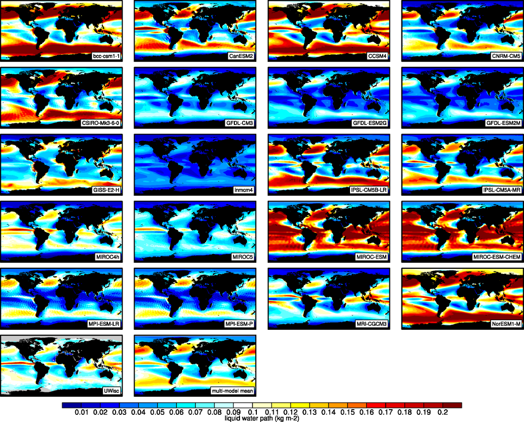
Fig. 4 The 20-yr average LWP (1986-2005) from the CMIP5 historical model runs and the multi-model mean in comparison with the UWisc satellite climatology (1988-2007) based on SSM/I, TMI, and AMSR-E (O’Dell et al. 2008).
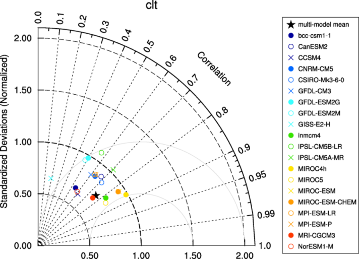
Fig. 5 Taylor diagram showing the 20-yr annual average performance of CMIP5 models for total cloud fraction as compared to MODIS satellite observations.
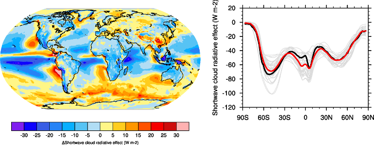
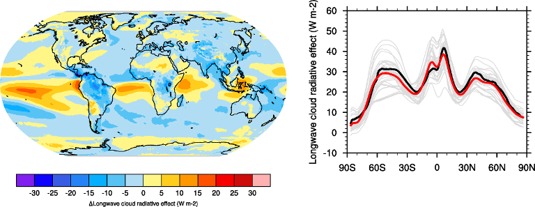
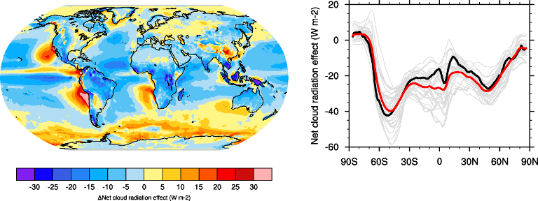
Fig. 6 20-year average (1986-2005) annual mean cloud radiative effects of CMIP5 models against the CERES EBAF (2001–2012). Top row shows the shortwave effect; middle row the longwave effect, and bottom row the net effect. Multi-model mean biases against CERES EBAF are shown on the left, whereas the right panels show zonal averages from CERES EBAF (thick black), the individual CMIP5 models (thin gray lines) and the multi-model mean (thick red line). Similar to Figure 9.5 of Flato et al. (2013).
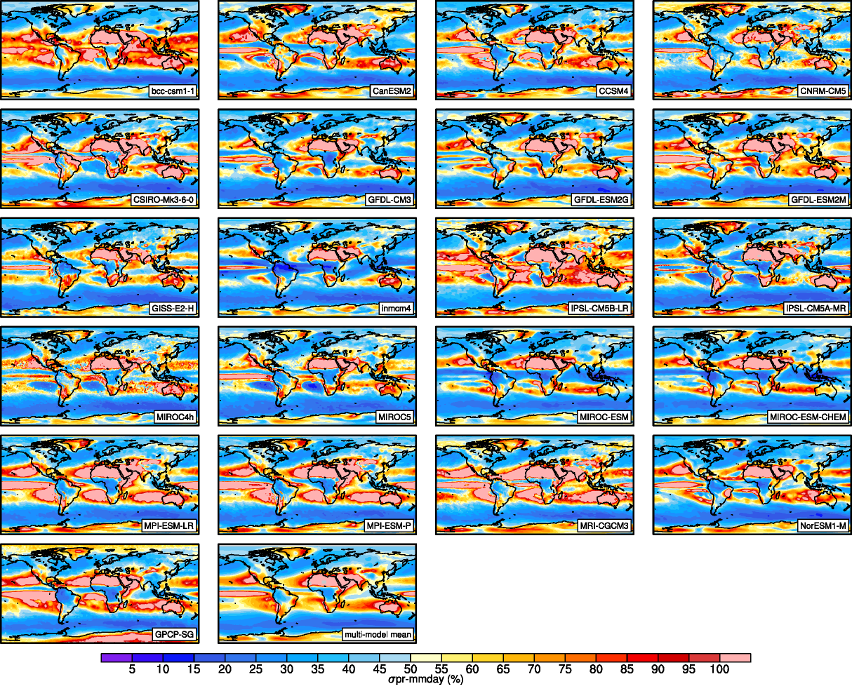
Fig. 7 Interannual variability of modeled and observed (GPCP) precipitation rates estimated as relative temporal standard deviation from 20 years (1986-2005) of data. The temporal standard devitions are calculated from monthly anomalies after subtracting the climatological mean seasonal cycle.