Quantifying progress across different CMIP phases
Overview
The recipe recipe_bock20jgr.yml generates figures to quantify the progress across different CMIP phases.
Note
The current recipe uses a horizontal 5x5 grid for figure 10, while the original plot in the paper shows a 2x2 grid. This is solely done for computational reasons (running the recipe with a 2x2 grid for figure 10 takes considerably more time than running it with a 5x5 grid) and can be easily changed in the preprocessor section of the recipe if necessary.
Available recipes and diagnostics
Recipes are stored in recipes/bock20jgr
recipe_bock20jgr_fig_1-4.yml
recipe_bock20jgr_fig_6-7.yml
recipe_bock20jgr_fig_8-10.yml
Diagnostics are stored in diag_scripts/
Fig. 1:
bock20jgr/tsline.ncl: timeseries of global mean surface temperature anomalies
Fig. 2:
bock20jgr/tsline_collect.ncl: collect different timeseries from tsline.ncl to compare different models ensembles
Fig. 3 and 4:
bock20jgr/model_bias.ncl: global maps of the multi-model mean and the multi-model mean bias
Fig. 6:
perfmetrics/main.ncl
perfmetrics/collect.ncl
Fig. 7:
bock20jgr/corr_pattern.ncl: calculate pattern correlation
bock20jgr/corr_pattern_collect.ncl: create pattern correlation plot
Fig. 8:
climate_metrics/ecs.py
climate_metrics/create_barplot.py
Fig. 9:
clouds/clouds_ipcc.ncl
Fig. 10:
climate_metrics/feedback_parameters.py
User settings in recipe
Script tsline.ncl
Required settings (scripts)
styleset: as in diag_scripts/shared/plot/style.ncl functions
Optional settings (scripts)
time_avg: type of time average (currently only “yearly” and “monthly” are available).
ts_anomaly: calculates anomalies with respect to the defined reference period; for each gird point by removing the mean for the given calendar month (requiring at least 50% of the data to be non-missing)
ref_start: start year of reference period for anomalies
ref_end: end year of reference period for anomalies
ref_value: if true, right panel with mean values is attached
ref_mask: if true, model fields will be masked by reference fields
region: name of domain
plot_units: variable unit for plotting
y_min: set min of y-axis
y_max: set max of y-axis
mean_nh_sh: if true, calculate first NH and SH mean
volcanoes: if true, lines of main volcanic eruptions will be added
header: if true, use region name as header
write_stat: if true, write multi-model statistics to nc-file
Required settings (variables)
none
Optional settings (variables)
none
Script tsline_collect.ncl
Required settings (scripts)
styleset: as in diag_scripts/shared/plot/style.ncl functions
Optional settings (scripts)
time_avg: type of time average (currently only “yearly” and “monthly” are available).
ts_anomaly: calculates anomalies with respect to the defined period
ref_start: start year of reference period for anomalies
ref_end: end year of reference period for anomalies
region: name of domain
plot_units: variable unit for plotting
y_min: set min of y-axis
y_max: set max of y-axis
order: order in which experiments should be plotted
header: if true, region name as header
stat_shading: if true: shading of statistic range
ref_shading: if true: shading of reference period
Required settings (variables)
none
Optional settings (variables)
none
Script model_bias.ncl
Required settings (scripts)
none
Optional settings (scripts)
projection: map projection, e.g., Mollweide, Mercator
timemean: time averaging, i.e. “seasonalclim” (DJF, MAM, JJA, SON), “annualclim” (annual mean)
Required settings (variables)*
reference_dataset: name of reference datatset
Optional settings (variables)
long_name: description of variable
Color tables
variable “tas”: diag_scripts/shared/plot/rgb/ipcc-ar6_temperature_div.rgb,
variable “pr-mmday”: diag_scripts/shared/plots/rgb/ipcc-ar6_precipitation_seq.rgb diag_scripts/shared/plot/rgb/ipcc-ar6_precipitation_div.rgb
Script perfmetrics_main.ncl
See here.
Script perfmetrics_collect.ncl
See here.
Script corr_pattern.ncl
Required settings (scripts)
none
Optional settings (scripts)
plot_median
Required settings (variables)
reference_dataset
Optional settings (variables)
alternative_dataset
Script corr_pattern_collect.ncl
Required settings (scripts)
none
Optional settings (scripts)
diag_order
Color tables
diag_scripts/shared/plot/rgb/ipcc-ar6_line_03.rgb
Script ecs.py
See here.
Script create_barplot.py
See here.
Script clouds_ipcc.ncl
See here.
Script feedback_parameters.py
Required settings (scripts)
none
Optional settings (scripts)
calculate_mmm: bool (default:
True). Calculate multi-model means.only_consider_mmm: bool (default:
False). Only consider multi-model mean dataset. This automatically setscalculate_mmmtoTrue. For large multi-dimensional datasets, this might significantly reduce the computation time if only the multi-model mean dataset is relevant.output_attributes: dict. Write additional attributes to netcdf files.
seaborn_settings: dict. Options for
seaborn.set()(affects all plots).
Variables
clt (atmos, monthly, longitude latitude time)
hus (atmos, monthly, longitude latitude lev time)
pr (atmos, monthly, longitude latitude time)
psl (atmos, monthly, longitude latitude time)
rlut (atmos, monthly, longitude latitude time)
rsdt (atmos, monthly, longitude latitude time)
rsut (atmos, monthly, longitude latitude time)
rtmt (atmos, monthly, longitude latitude time)
rlutcs (atmos, monthly, longitude latitude time)
rsutcs (atmos, monthly, longitude latitude time)
ta (atmos, monthly, longitude latitude lev time)
tas (atmos, monthly, longitude latitude time)
ts (atmos, monthly, longitude latitude time)
ua (atmos, monthly, longitude latitude lev time)
va (atmos, monthly, longitude latitude lev time)
zg (atmos, monthly, longitude latitude time)
Observations and reformat scripts
AIRS (obs4MIPs) - specific humidity
CERES-EBAF (obs4MIPs) - CERES TOA radiation fluxes (used for calculation of cloud forcing)
ERA-Interim - reanalysis of surface temperature, sea surface pressure
Reformat script: recipes/cmorizers/recipe_era5.yml
ERA5 - reanalysis of surface temperature
Reformat script: recipes/cmorizers/recipe_era5.yml
ESACCI-CLOUD - total cloud cover
Reformat script: cmorizers/data/formatters/datasets/esacci_cloud.ncl
ESACCI-SST - sea surface temperature
Reformat script: cmorizers/data/formatters/datasets/esacci_sst.py
GHCN - Global Historical Climatology Network-Monthly gridded land precipitation
Reformat script: cmorizers/data/formatters/datasets/ghcn.ncl
GPCP-SG (obs4MIPs) - Global Precipitation Climatology Project total precipitation
HadCRUT4 - surface temperature anomalies
Reformat script: cmorizers/data/formatters/datasets/hadcrut4.ncl
HadISST - surface temperature
Reformat script: cmorizers/data/formatters/datasets/hadisst.ncl
JRA-55 (ana4mips) - reanalysis of sea surface pressure
NCEP - reanalysis of surface temperature
Reformat script: cmorizers/data/formatters/datasets/ncep.ncl
PATMOS-x - total cloud cover
Reformat script: cmorizers/data/formatters/datasets/patmos_x.ncl
References
Bock, L., Lauer, A., Schlund, M., Barreiro, M., Bellouin, N., Jones, C., Predoi, V., Meehl, G., Roberts, M., and Eyring, V.: Quantifying progress across different CMIP phases with the ESMValTool, Journal of Geophysical Research: Atmospheres, 125, e2019JD032321. https://doi.org/10.1029/2019JD032321
Copernicus Climate Change Service (C3S), 2017: ERA5: Fifth generation of ECMWF atmospheric reanalyses of the global climate, edited, Copernicus Climate Change Service Climate Data Store (CDS). https://cds.climate.copernicus.eu/cdsapp#!/home
Flato, G., J. Marotzke, B. Abiodun, P. Braconnot, S.C. Chou, W. Collins, P. Cox, F. Driouech, S. Emori, V. Eyring, C. Forest, P. Gleckler, E. Guilyardi, C. Jakob, V. Kattsov, C. Reason and M. Rummukainen, 2013: Evaluation of Climate Models. In: Climate Change 2013: The Physical Science Basis. Contribution of Working Group I to the Fifth Assessment Report of the Intergovernmental Panel on Climate Change [Stocker, T.F., D. Qin, G.-K. Plattner, M. Tignor, S.K. Allen, J. Boschung, A. Nauels, Y. Xia, V. Bex and P.M. Midgley (eds.)]. Cambridge University Press, Cambridge, United Kingdom and New York, NY, USA.
Morice, C. P., Kennedy, J. J., Rayner, N. A., & Jones, P., 2012: Quantifying uncertainties in global and regional temperature change using an ensemble of observational estimates: The HadCRUT4 data set, Journal of Geophysical Research, 117, D08101. https://doi.org/10.1029/2011JD017187
Example plots

Fig. 37 Observed and simulated time series of the anomalies in annual and global mean surface temperature. All anomalies are differences from the 1850-1900 time mean of each individual time series (Fig. 1).
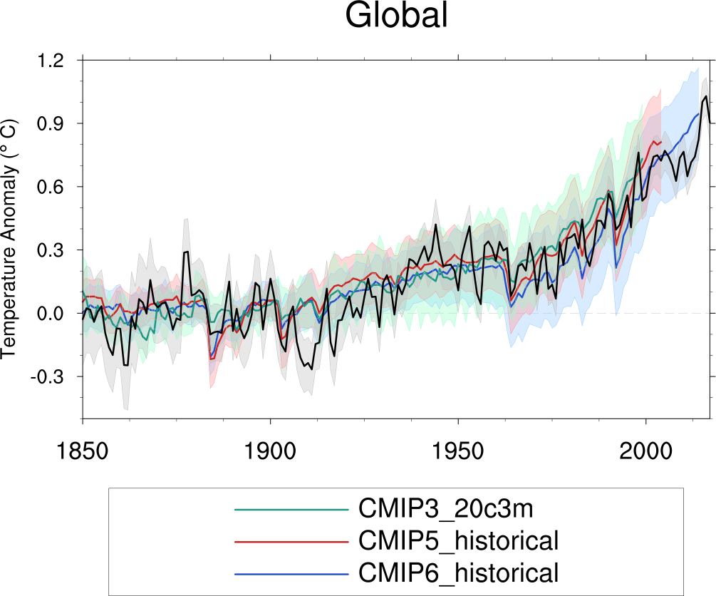
Fig. 38 Observed and simulated time series of the anomalies in annual and global mean surface temperature as in Figure 1; all anomalies are calculated by subtracting the 1850-1900 time mean from the time series. Displayed are the multimodel means of all three CMIP ensembles with shaded range of the respective standard deviation. In black the HadCRUT4 data set (HadCRUT4; Morice et al., 2012). Gray shading shows the 5% to 95% confidence interval of the combined effects of all the uncertainties described in the HadCRUT4 error model (measurement and sampling, bias, and coverage uncertainties) (Morice et al., 2012) (Fig. 2).
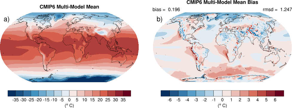
Fig. 39 Annual mean near‐surface (2 m) air temperature (°C). (a) Multimodel (ensemble) mean constructed with one realization of CMIP6 historical experiments for the period 1995-2014. Multimodel‐mean bias of (b) CMIP6 (1995-2014) compared to the corresponding time period of the climatology from ERA5 (Copernicus Climate Change Service (C3S), 2017). (Fig. 3)
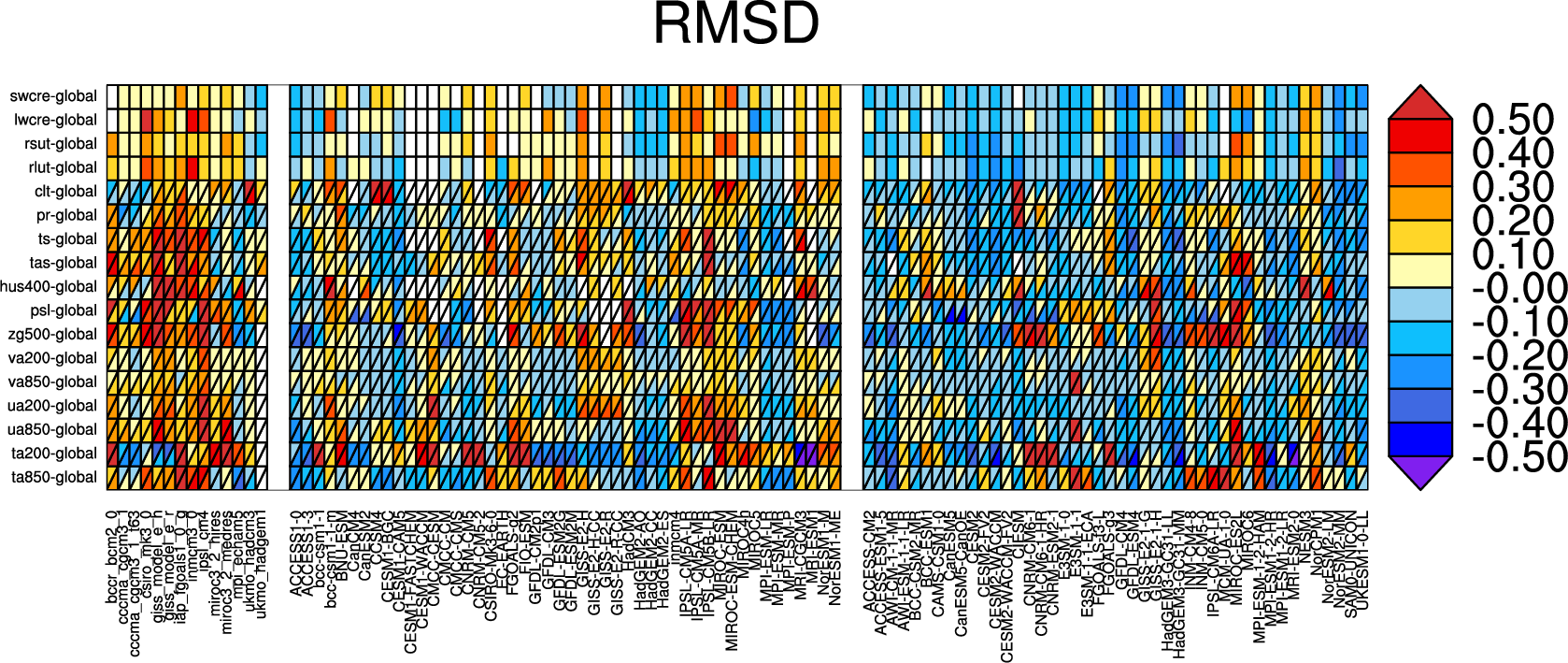
Fig. 40 Relative space-time root-mean-square deviation (RMSD) calculated from the climatological seasonal cycle of the CMIP3, CMIP5, and CMIP6 simulations (1980-1999) compared to observational data sets (Table 5). A relative performance is displayed, with blue shading being better and red shading worse than the median RMSD of all model results of all ensembles. A diagonal split of a grid square shows the relative error with respect to the reference data set (lower right triangle) and the alternative data set (upper left triangle) which are marked in Table 5. White boxes are used when data are not available for a given model and variable (Fig. 6).
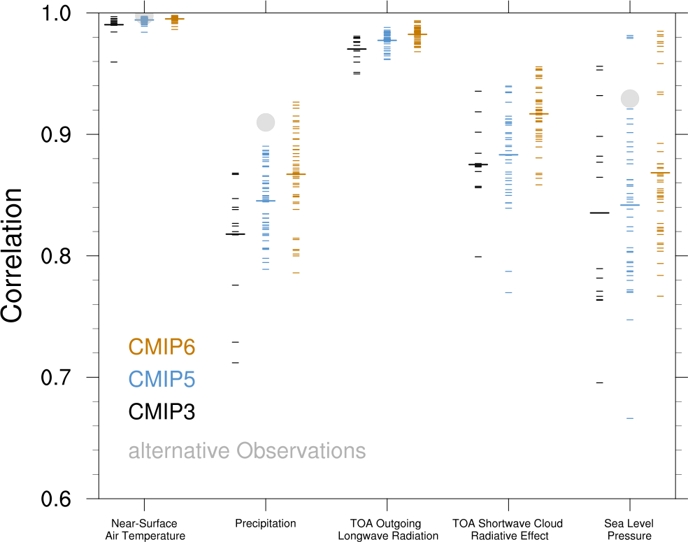
Fig. 41 Centered pattern correlations between models and observations for the annual mean climatology over the period 1980–1999 (Fig. 7).