Blocking metrics and indices, teleconnections and weather regimes (MiLES)
Overview
Atmospheric blocking is a recurrent mid-latitude weather pattern identified by a large-amplitude, quasi-stationary, long-lasting, high-pressure anomaly that ‘‘blocks’’ the westerly flow forcing the jet stream to split or meander (Rex, 1950).
It is typically initiated by the breaking of a Rossby wave in a diffluence region at the exit of the storm track, where it amplifies the underlying stationary ridge (Tibaldi and Molteni, 1990). Blocking occurs more frequently in the Northern Hemisphere cold season, with larger frequencies observed over the Euro-Atlantic and North Pacific sectors. Its lifetime oscillates from a few days up to several weeks (Davini et al., 2012) sometimes leading to winter cold spells or summer heat waves.
To this end, the MId-Latitude Evaluation System (MiLES) was developed as stand-alone package (https://github.com/oloapinivad/MiLES) to support analysis of mid-latitude weather patterns in terms of atmospheric blocking, teleconnections and weather regimes. The package was then implemented as recipe for ESMValTool.
The tool works on daily 500hPa geopotential height data (with data interpolated on a common 2.5x2.5 grid) and calculates the following diagnostics:
1D Atmospheric Blocking
Tibaldi and Molteni (1990) index for Northern Hemisphere. Computed at fixed latitude of 60N, with delta of -5,-2.5,0,2.5,5 deg, fiN=80N and fiS=40N. Full timeseries and climatologies are provided in NetCDF4 Zip format.
2D Atmospheric blocking
Following the index by Davini et al. (2012). It is a 2D version of Tibaldi and Molteni (1990) for Northern Hemisphere atmospheric blocking evaluating meridional gradient reversal at 500hPa. It computes both Instantaneous Blocking and Blocking Events frequency, where the latter allows the estimation of the each blocking duration. It includes also two blocking intensity indices, i.e. the Meridional Gradient Index and the Blocking Intensity index. In addition the orientation (i.e. cyclonic or anticyclonic) of the Rossby wave breaking is computed. A supplementary Instantaneous Blocking index with the GHGS2 condition (see Davini et al., 2012) is also evaluated. Full timeseries and climatologies are provided in NetCDF4 Zip format.
Z500 Empirical Orthogonal Functions
Based on SVD. The first 4 EOFs for North Atlantic (over the 90W-40E 20N-85N box) and Northern Hemisphere (20N-85N) or a custom region are computed. North Atlantic Oscillation, East Atlantic Pattern, and Arctic Oscillation can be evaluated. Figures showing linear regression of PCs on monthly Z500 are provided. PCs and eigenvectors, as well as the variances explained are provided in NetCDF4 Zip format.
North Atlantic Weather Regimes
Following k-means clustering of 500hPa geopotential height. 4 weather regimes over North Atlantic (80W-40E 30N-87.5N) are evaluated using anomalies from daily seasonal cycle. This is done retaining the first North Atlantic EOFs which explains the 80% of the variance to reduce the phase-space dimensions and then applying k-means clustering using Hartigan-Wong algorithm with k=4. Figures report patterns and frequencies of occurrence. NetCDF4 Zip data are saved. Only 4 regimes and DJF supported so far.
Available recipes and diagnostics
Recipes are stored in recipes/
recipe_miles_block.yml
recipe_miles_eof.yml
recipe_miles_regimes.yml
Diagnostics are stored in diag_scripts/miles/
miles_block.R
miles_eof.R
miles_regimes.R
and subroutines
basis_functions.R
block_figures.R
eof_figures.R
regimes_figures.R
block_fast.R
eof_fast.R
miles_parameters.R
regimes_fast.R
miles_parameters.R contains additional internal parameters which affect plot sizes, colortables etc.
User settings
miles_block.R
Required settings for variables
reference_dataset: reference dataset for comparison
reference_exp: optional reference experiment for comparison (to use when comparing two experiments of the same dataset)
Required settings for script
seasons: Selected season(‘DJF’,’MAM’,’JJA’,’SON’,’ALL’) or your period as e.g. ‘Jan_Feb_Mar’
miles_eof.R
Required settings for variables
reference_dataset: reference dataset for comparison
reference_exp: optional reference experiment for comparison (to use when comparing two experiments of the same dataset)
Required settings for script
seasons: Selected season(‘DJF’,’MAM’,’JJA’,’SON’,’ALL’) or your period as e.g. ‘Jan_Feb_Mar’
teles: Select EOFs (‘NAO’,’AO’,’PNA’) or specify custom area as “lon1_lon2_lat1_lat2”
miles_regimes.R
Required settings for variables
reference_dataset: reference dataset
reference_exp: optional reference experiment for comparison (to use when comparing two experiments of the same dataset)
Required or optional settings for script
None (the two parameters seasons and nclusters in the recipe should not be changed)
Variables
zg (atmos, daily mean, longitude latitude time)
Observations and reformat scripts
ERA-INTERIM
References
REX, D. F. (1950), Blocking Action in the Middle Troposphere and its Effect upon Regional Climate. Tellus, 2: 196-211. doi: http://doi.org/10.1111/j.2153-3490.1950.tb00331.x
Davini, P., C. Cagnazzo, S. Gualdi, and A. Navarra (2012): Bidimensional Diagnostics, Variability, and Trends of Northern Hemisphere Blocking. J. Climate, 25, 6496–6509, doi: http://doi.org/10.1175/JCLI-D-12-00032.1.
Tibaldi S, Molteni F.: On the operational predictability of blocking. Tellus A 42(3): 343–365, doi: 10.1034/j.1600- 0870.1990.t01- 2- 00003.x, 1990. https://doi.org/10.1034/j.1600-0870.1990.t01-2-00003.x
Paolo Davini. (2018, April 30). MiLES - Mid Latitude Evaluation System (Version v0.51). Zenodo. http://doi.org/10.5281/zenodo.1237838
Example plots
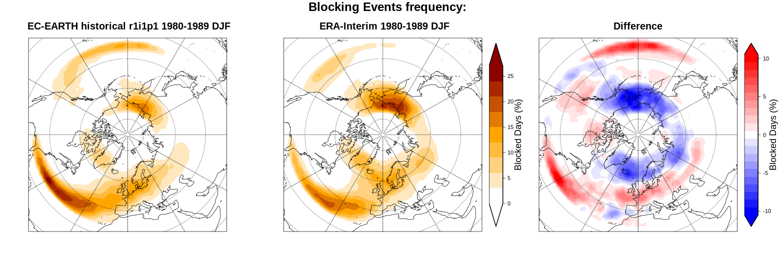
Fig. 2 Blocking Events frequency for a CMIP5 EC-Earth historical run (DJF 1980-1989), compared to ERA-Interim. Units are percentage of blocked days per season.
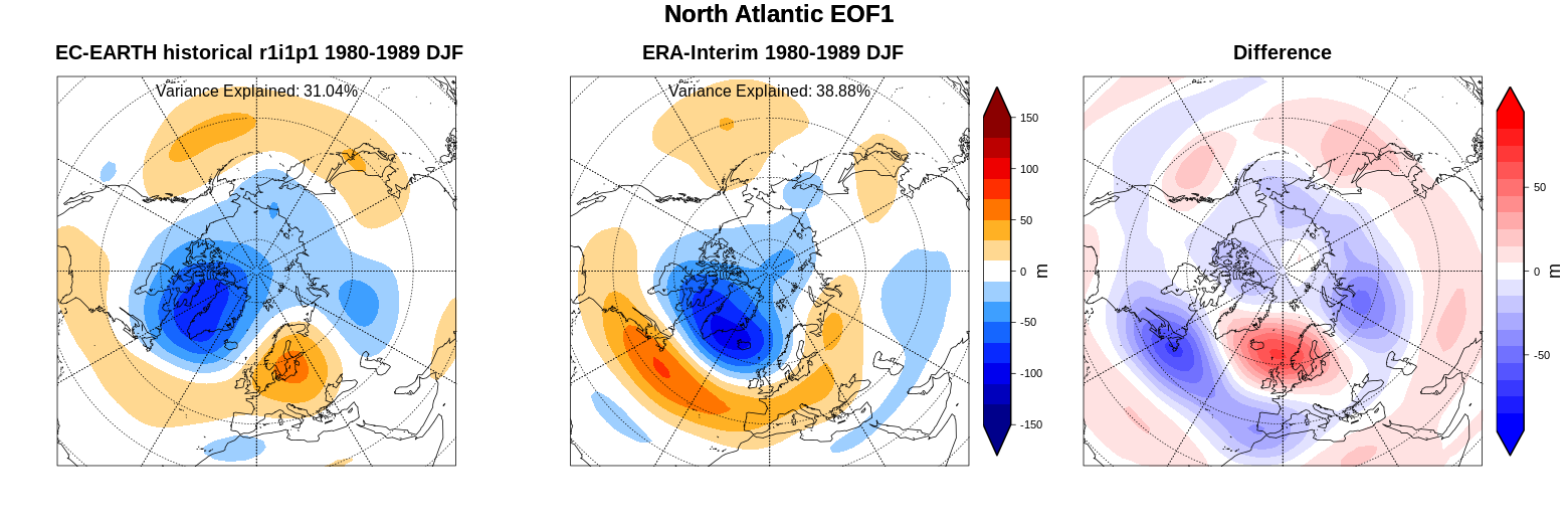
Fig. 3 North Atlantic Oscillation for a CMIP5 EC-Earth historical run (DJF 1980-1989) compared to ERA-Interim, shown as the linear regression of the monthly Z500 against the first Principal Component (PC1) of the North Atlantic region.