KNMI Climate Scenarios 2014
Overview
This recipe implements the method described in Lenderink et al., 2014, to prepare the 2014 KNMI Climate Scenarios (KCS) for the Netherlands. A set of 8 global climate projections from EC-Earth were downscaled with the RACMO regional climate model. Since the EC-Earth ensemble is not readily representative for the spread in the full CMIP ensemble, this method recombines 5-year segments from the EC-Earth ensemble to obtain a large suite of “resamples”. Subsequently, 8 new resamples are selected that cover the spread in CMIP much better than the original set.
The original method created 8 resampled datasets:
2 main scenarios: Moderate (M) and Warm (W) (Lenderink 2014 uses “G” instead of “M”).
2 ‘sub’scenarios: Relatively high (H) or low (L) changes in seasonal temperature and precipitation
2 time horizons: Mid-century (MOC; 2050) and end-of-century (EOC; 2085)
Each scenario consists of changes calculated between 2 periods: Control (e.g. 1981-2010) and future (variable).
The configuration settings for these resamples can be found in table 1 of Lenderink 2014’s supplementary data.
Implementation
The implementation is such that application to other datasets, regions, etc. is relatively straightforward. The description below focuses on the reference use case of Lenderink et al., 2014, where the target model was EC-Earth. An external set of EC-Earth data (all RCP85) was used, for which 3D fields for downscaling were available as well. In the recipe shipped with ESMValTool, however, the target model is CCSM4, so that it works out of the box with ESGF data only.
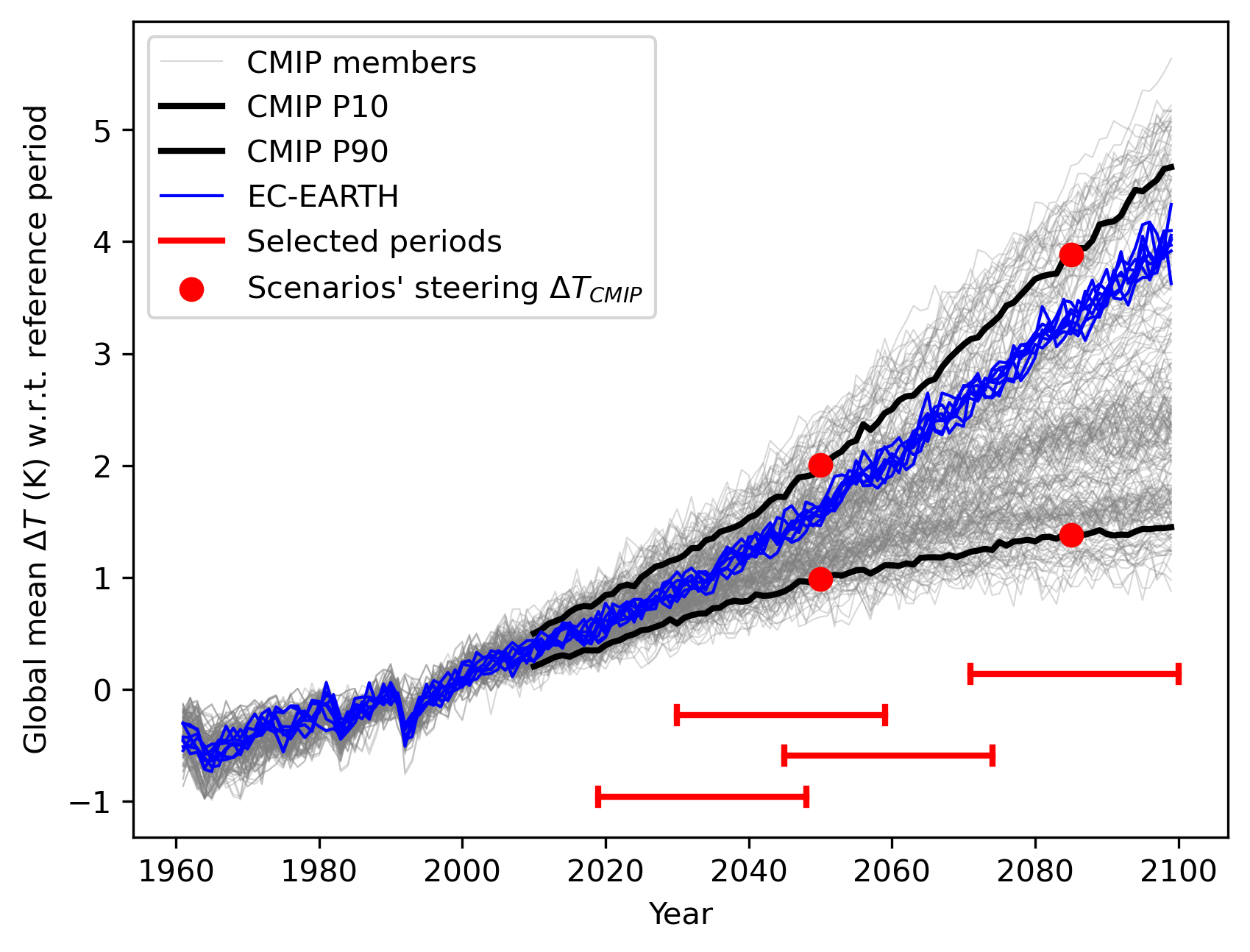
In the first diagnostic, the spread of the full CMIP ensemble is used to obtain 4 values of a global \({\Delta}T_{CMIP}\), corresponding to the 10th and 90th percentiles for the M and W scenarios, respectively, for both MOC and EOC. Subsequently, for each of these 4 steering parameters, 30-year periods are selected from the target model ensemble, where \({\Delta}T_{target}{\approx}{\Delta}T_{CMIP}\).
In the second diagnostic, for both the control and future periods, the N target model ensemble members are split into 6 segments of 5 years each. Out of all \(N^6\) possible re-combinations of these 5-year segments, eventually M new ‘resamples’ are selected based on local changes in seasonal temperature and precipitation. This is done in the following steps:
Select 1000 samples for the control period, and 2 x 1000 samples for the future period (one for each subscenario). Step 1 poses a constraint on winter precipitation. For the control period, winter precipitation must still closely represent the average of the original ensemble. For the two future periods, the change in winter precipitation with respect to the control period must approximately equal 4% per degree \({\Delta}T\) (subscenario L) or 8% per degree \({\Delta}T\) (subscenario H).
Further constrain the selection by picking samples that represent either high or low changes in summer precipitation and summer and winter temperature, by limiting the remaining samples to certain percentile ranges: relatively wet/cold in the control and dry/warm in the future, or vice versa. The percentile ranges are listed in table 1 of Lenderink 2014’s supplement. This should result is approximately 50 remaining samples for each scenario, for both control and future.
Use a Monte-Carlo method to make a final selection of 8 resamples with minimal reuse of the same ensemble member/segment.
Datasets have been split in two parts: the CMIP datasets and the target model datasets. An example use case for this recipe is to compare between CMIP5 and CMIP6, for example. The recipe can work with a target model that is not part of CMIP, provided that the data are CMOR compatible, and using the same data referece syntax as the CMIP data. Note that you can specify multiple data paths in the user configuration file.
Available recipes and diagnostics
Recipes are stored in recipes/
recipe_kcs.yml
Diagnostics are stored in diag_scripts/kcs/
global_matching.py
local_resampling.py
Note
We highly recommend using the options described in Re-running diagnostics. The speed bottleneck for the first diagnostic is the preprocessor. In the second diagnostic, step 1 is most time consuming, whereas steps 2 and 3 are likely to be repeated several times. Therefore, intermediate files are saved after step 1, and the diagnostic will automatically detect and use them if the -i flag is used.
User settings
Script <global_matching.py>
Required settings for script
scenario_years: a list of time horizons. Default:[2050, 2085]
scenario_percentiles: a list of percentiles for the steering table. Default:[p10, p90]Required settings for preprocessor This diagnostic needs global mean temperature anomalies for each dataset, both CMIP and the target model. Additionally, the multimodel statistics preprocessor must be used to produce the percentiles specified in the setting for the script above.
Script <local_resampling.py>
Required settings for script
control_period: the control period shared between all scenarios. Default:[1981, 2010]
n_samples: the final number of recombinations to be selected. Default:8
scenarios: a scenario name and list of options. The default setting is a single scenario:scenarios: ML_MOC: # scenario name; can be chosen by the user description: "Moderate / low changes in seasonal temperature & precipitation" global_dT: 1.0 scenario_year: 2050 resampling_period: [2021, 2050] dpr_winter: 4 pr_summer_control: [25, 55] pr_summer_future: [45, 75] tas_winter_control: [50, 80] tas_winter_future: [20, 50] tas_summer_control: [0, 100] tas_summer_future: [0, 50]These values are taken from table 1 in the Lenderink 2014’s supplementary material. Multiple scenarios can be processed at once by appending more configurations below the default one. For new applications,
global_dT,resampling_periodanddpr_winterare informed by the output of the first diagnostic. The percentile bounds in the scenario settings (e.g.tas_winter_controlandtas_winter_future) are to be tuned until a satisfactory scenario spread over the full CMIP ensemble is achieved.Required settings for preprocessor
This diagnostic requires data on a single point. However, the
extract_pointpreprocessor can be changed toextract_shapeorextract_region, in conjunction with an area mean. And of course, the coordinates can be changed to analyze a different region.
Variables
Variables are precipitation and temperature, specified separately for the target model and the CMIP ensemble:
pr_target (atmos, monthly mean, longitude latitude time)
tas_target (atmos, monthly mean, longitude latitude time)
pr_cmip (atmos, monthly mean, longitude latitude time)
tas_cmip (atmos, monthly mean, longitude latitude time)
Example output
The diagnostic global_matching produces a scenarios table like the one below
   year percentile  cmip_dt period_bounds  target_dt  pattern_scaling_factor
0  2050        P10     0.98  [2019, 2048]       0.99                    1.00
1  2050        P90     2.01  [2045, 2074]       2.02                    0.99
2  2085        P10     1.38  [2030, 2059]       1.38                    1.00
3  2085        P90     3.89  [2071, 2100]       3.28                    1.18
which is printed to the log file and also saved as a csv-file scenarios.csv.
Additionally, a figure is created showing the CMIP spread in global temperature change,
AND highlighting the selected steering parameters and resampling periods:
The diagnostic local_resampling procudes a number of output files:
season_means_<scenario>.nc: intermediate results, containing the season means for each segment of the original target model ensemble.top1000_<scenario>.csv: intermediate results, containing the 1000 combinations that have been selected based on winter mean precipitation.indices_<scenario>.csv: showing the final set of resamples as a table:control future Segment 0 Segment 1 Segment 2 Segment 3 Segment 4 Segment 5 Segment 0 Segment 1 Segment 2 Segment 3 Segment 4 Segment 5 Combination 0 5 7 6 3 1 3 2 4 2 4 7 7 Combination 1 0 3 0 4 3 2 4 1 6 1 3 0 Combination 2 2 4 3 7 4 2 5 4 6 6 4 2 Combination 3 1 4 7 2 3 6 5 3 1 7 4 1 Combination 4 5 7 6 3 1 3 2 3 0 6 1 7 Combination 5 7 2 1 4 5 1 6 0 4 2 3 3 Combination 6 7 2 2 0 6 6 5 2 1 5 4 2 Combination 7 6 3 2 1 6 1 2 1 0 2 1 3
resampled_control_<scenario>.nc: containing the monthly means for the control period according to the final combinations.resampled_future_<scenario>.nc: containing the monthly means for the future period according to the final combinations.Provenance information: bibtex, xml, and/or text files containing citation information are stored alongside the final result and the final figure. The final combinations only derive from the target model data, whereas the figure also uses CMIP data.
A figure used to validate the final result, reproducing figures 5 and 6 from Lenderink et al.:
