Modes of variability
Overview
The goal of this recipe is to compute modes of variability from a reference or observational dataset and from a set of climate projections and calculate the root-mean-square error between the mean anomalies obtained for the clusters from the reference and projection data sets. This is done through K-means or hierarchical clustering applied either directly to the spatial data or after computing the EOFs.
The user can specify the number of clusters to be computed.
The recipe’s output consist of three netcdf files for both the observed and projected weather regimes and the RMSE between them.
Available recipes and diagnostics
Recipes are stored in recipes/
recipe_modes_of_variability.yml
Diagnostics are stored in diag_scripts/magic_bsc/
WeatherRegime.R - function for computing the EOFs and k-means and hierarchical clusters.
weather_regime.R - applies the above weather regimes function to the datasets
User settings
User setting files are stored in recipes/
recipe_modes_of_variability.yml
Required settings for script
plot type: rectangular or polar
ncenters: number of centers to be computed by the clustering algorithm (maximum 4)
cluster_method: kmeans (only psl variable) or hierarchical clustering (for psl or sic variables)
detrend_order: the order of the polynomial detrending to be applied (0, 1 or 2)
EOFs: logical indicating wether the k-means clustering algorithm is applied directly to the spatial data (‘false’) or to the EOFs (‘true’)
frequency: select the month (format: JAN, FEB, …) or season (format: JJA, SON, MAM, DJF) for the diagnostic to be computed for (does not work yet for MAM with daily data).
Variables
psl (atmos, monthly/daily, longitude, latitude, time)
Observations and reformat scripts
None
References
Dawson, A., T. N. Palmer, and S. Corti, 2012: Simulating regime structures in weather and climate prediction models. Geophysical Research Letters, 39 (21), https://doi.org/10.1029/2012GL053284.
Ferranti, L., S. Corti, and M. Janousek, 2015: Flow-dependent verification of the ECMWF ensemble over the Euro-Atlantic sector. Quarterly Journal of the Royal Meteorological Society, 141 (688), 916-924, https://doi.org/10.1002/qj.2411.
Grams, C. M., Beerli, R., Pfenninger, S., Staffell, I., & Wernli, H. (2017). Balancing Europe’s wind-power output through spatial deployment informed by weather regimes. Nature climate change, 7(8), 557, https://doi.org/10.1038/nclimate3338.
Hannachi, A., D. M. Straus, C. L. E. Franzke, S. Corti, and T. Woollings, 2017: Low Frequency Nonlinearity and Regime Behavior in the Northern Hemisphere Extra-Tropical Atmosphere. Reviews of Geophysics, https://doi.org/10.1002/2015RG000509.
Michelangeli, P.-A., R. Vautard, and B. Legras, 1995: Weather regimes: Recurrence and quasi stationarity. Journal of the atmospheric sciences, 52 (8), 1237-1256, doi: 10.1175/1520-0469(1995)052<1237:WRRAQS>2.0.CO.
Vautard, R., 1990: Multiple weather regimes over the North Atlantic: Analysis of precursors and successors. Monthly weather review, 118 (10), 2056-2081, doi: 10.1175/1520-0493(1990)118<2056:MWROTN>2.0.CO;2.
Yiou, P., K. Goubanova, Z. X. Li, and M. Nogaj, 2008: Weather regime dependence of extreme value statistics for summer temperature and precipitation. Nonlinear Processes in Geophysics, 15 (3), 365-378, https://doi.org/10.5194/npg-15-365-2008.
Example plots
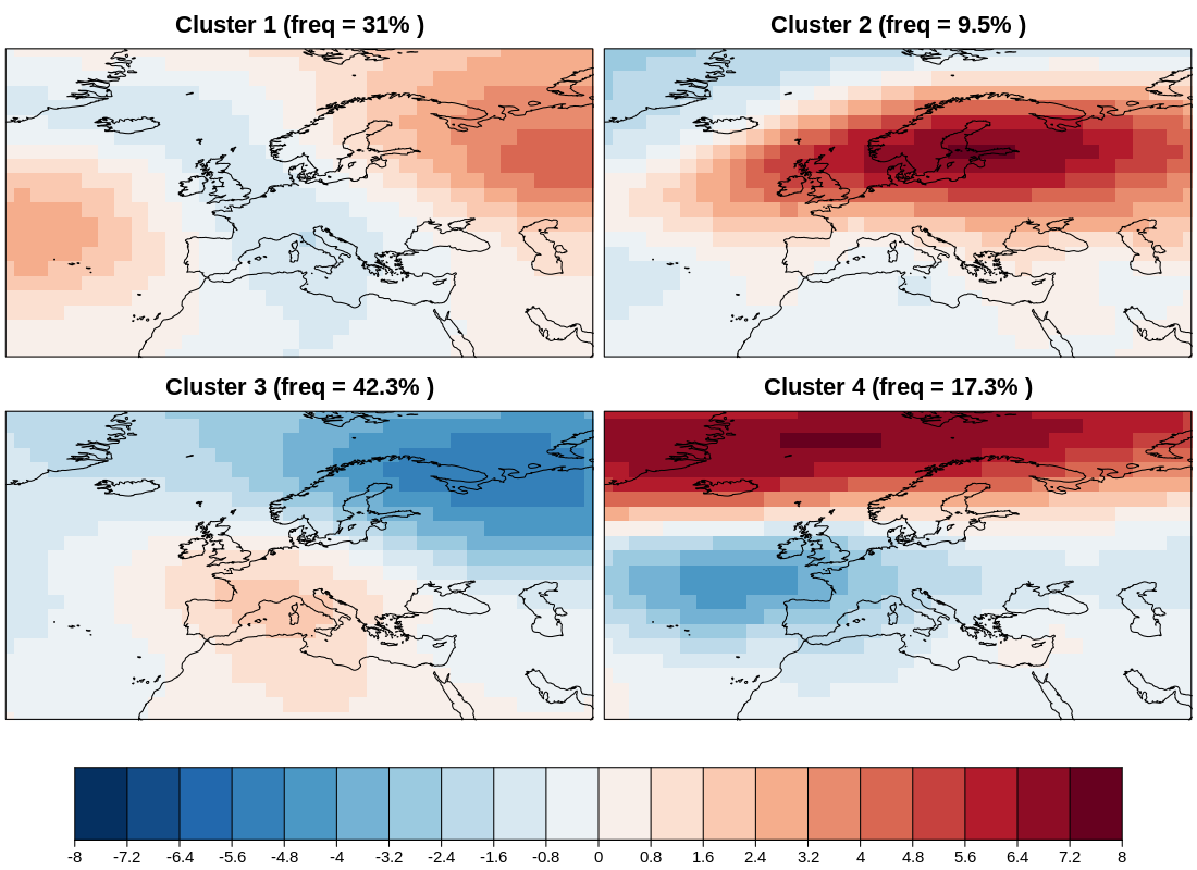
Four modes of variability for autumn (September-October-November) in the North Atlantic European Sector for the RCP 8.5 scenario using BCC-CSM1-1 future projection during the period 2020-2075. The frequency of occurrence of each variability mode is indicated in the title of each map.