Ocean metrics
Overview
The Southern Ocean is central to the global climate and the global carbon cycle, and to the climate’s response to increasing levels of atmospheric greenhouse gases. Global coupled climate models and earth system models, however, vary widely in their simulations of the Southern Ocean and its role in, and response to, the ongoing anthropogenic trend. Observationally-based metrics are critical for discerning processes and mechanisms, and for validating and comparing climate and earth system models. New observations and understanding have allowed for progress in the creation of observationally-based data/model metrics for the Southern Ocean.
The metrics presented in this recipe provide a means to assess multiple simulations relative to the best available observations and observational products. Climate models that perform better according to these metrics also better simulate the uptake of heat and carbon by the Southern Ocean. Russell et al. 2018 assessed only a few of the available CMIP5 simulations, but most of the available CMIP5 and CMIP6 climate models can be analyzed with these recipes.
The goal is to create a recipe for recreation of metrics in Russell, J.L., et al., 2018, J. Geophys. Res. – Oceans, 123, 3120-3143, doi: 10.1002/2017JC013461.
Available recipes and diagnostics
Recipes are stored in recipes/
recipe_russell18jgr.yml
Diagnostics are stored in diag_scripts/russell18jgr/
russell18jgr-polar.ncl (figures 1, 7, 8): calculates and plots annual-mean variables (tauu, sic, fgco2, pH) as polar contour map.
russell18jgr-fig2.ncl: calculates and plots The zonal and annual means of the zonal wind stress (N/m2).
russell18jgr-fig3b.ncl: calculates and plots the latitudinal position of Subantarctic Front. Using definitions from Orsi et al (1995).
russell18jgr-fig3b-2.ncl: calculates and plots the latitudinal position of Polar Front. Using definitions from Orsi et al (1995).
russell18jgr-fig4.ncl: calculates and plots the zonal velocity through Drake Passage (at 69W) and total transport through the passage if the volcello file is available.
russell18jgr-fig5.ncl: calculates and plots the mean extent of sea ice for September(max) in blue and mean extent of sea ice for February(min) in red.
russell18jgr-fig5g.ncl: calculates and plots the annual cycle of sea ice area in southern ocean.
russell18jgr-fig6a.ncl: calculates and plots the density layer based volume transport(in Sv) across 30S based on the layer definitions in Talley (2008).
russell18jgr-fig6b.ncl: calculates and plots the Density layer based heat transport(in PW) across 30S based on the layer definitions in Talley (2008).
russell18jgr-fig7h.ncl: calculates and plots the zonal mean flux of fgco2 in gC/(yr * m2).
russell18jgr-fig7i.ncl: calculates and plots the cumulative integral of the net CO2 flux from 90S to 30S (in PgC/yr).
russell18jgr-fig9a.ncl: calculates and plots the scatter plot of the width of the Southern Hemisphere westerly wind band against the annual-mean integrated heat uptake south of 30S (in PW), along with the line of best fit.
russell18jgr-fig9b.ncl: calculates and plots the scatter plot of the width of the Southern Hemisphere westerly wind band against the annual-mean integrated carbon uptake south of 30S (in Pg C/yr), along with the line of best fit.
russell18jgr-fig9c.ncl: calculates and plots the scatter plot of the net heat uptake south of 30S (in PW) against the annual-mean integrated carbon uptake south of 30S (in Pg C/yr), along with the line of best fit.
User settings in recipe
Script russell18jgr-polar.ncl
Required settings (scripts)
styleset : CMIP5(recommended), default, etc.
ncdf : default(recommended), CMIP5, etc.
max_lat : -30.0
Optional settings (scripts)
grid_max : 0.4 (figure 1), 30 (figure 7), 8.2 (figure 8)
grid_min : -0.4 (figure 1), -30 (figure 7), 8.0 (figure 8)
grid_step : 0.1 (figure 1), 2.5 (figure 7), 0.1 (figure 8)
colormap : BlWhRe (figure 7)
colors : [[237.6, 237.6, 0.], [ 255, 255, 66.4], [255, 255, 119.6], [255, 255, 191.8], [223.8, 191.8, 223.8], [192.8, 127.5, 190.8], [161.6, 65.3, 158.6], [129.5, 1.0, 126.5] ] (figure 1) [[132,12,127], [147,5,153], [172,12,173], [195,33,196], [203,63,209], [215,89,225], [229,117,230], [243,129,238], [253,155,247], [255,178,254], [255,255,255], [255,255,255], [126,240,138], [134,234,138], [95,219,89], [57,201,54], [39,182,57], [33,161,36], [16,139,22], [0,123,10], [6,96,6], [12,77,9.0] ] (figure 8)
max_vert : 1 - 4 (user preference)
max_hori : 1 - 4 (user preference)
grid_color: blue4 (figure 8)
labelBar_end_type: ExcludeOuterBoxes (figure 1), both_triangle (figure 7, 8)
unitCorrectionalFactor: -3.154e+10 (figure 7)
new_units : “gC/ (m~S~2~N~ * yr)” (figure 7)
Required settings (variables)
additional_dataset: datasets to plot.
Optional settings (variables)
none
Script russell18jgr-fig2.ncl
Required settings (scripts)
styleset : CMIP5(recommended), default, etc.
ncdf : default(recommended), CMIP5, etc.
Optional settings (scripts)
none
Script russell18jgr-fig3b.ncl
Required settings (scripts)
styleset : CMIP5(recommended), default, etc.
ncdf : default(recommended), CMIP5, etc.
Optional settings (scripts)
none
Script russell18jgr-fig3b-2.ncl
Required settings (scripts)
styleset : CMIP5(recommended), default, etc.
ncdf : default(recommended), CMIP5, etc.
Optional settings (scripts)
none
Script russell18jgr-fig4.ncl
Required settings (scripts)
styleset : CMIP5(recommended), default, etc.
ncdf : default(recommended), CMIP5, etc.
Optional settings (scripts)
max_vert : 1 - 4 (user preference)
max_hori : 1 - 4 (user preference)
unitCorrectionalFactor: 100 (m/s to cm/s)
new_units : “cm/s”
Script russell18jgr-fig5.ncl
Required settings (scripts)
styleset : CMIP5(recommended), default, etc.
ncdf : default(recommended), CMIP5, etc.
max_lat : -45.0
Optional settings (scripts)
max_vert : 1 - 4 (user preference)
max_hori : 1 - 4 (user preference)
Script russell18jgr-fig5g.ncl
Required settings (scripts)
styleset : CMIP5(recommended), default, etc.
Optional settings (scripts)
none
Script russell18jgr-fig6a.ncl
Required settings (scripts)
styleset : CMIP5(recommended), default, etc.
ncdf : default(recommended), CMIP5, etc.
Optional settings (scripts)
none
Script russell18jgr-fig6b.ncl
Required settings (scripts)
styleset : CMIP5(recommended), default, etc.
ncdf : default(recommended), CMIP5, etc.
Optional settings (scripts)
none
Script russell18jgr-fig7h.ncl
Required settings (scripts)
styleset : CMIP5(recommended), default, etc.
ncdf : default(recommended), CMIP5, etc.
Optional settings (scripts)
none
Script russell18jgr-fig7i.ncl
Required settings (scripts)
styleset : CMIP5(recommended), default, etc.
ncdf : default(recommended), CMIP5, etc.
Optional settings (scripts)
none
Script russell18jgr-fig9a.ncl
Required settings (scripts)
styleset : CMIP5(recommended), default, etc.
ncdf : default(recommended), CMIP5, etc.
Optional settings (scripts)
none
Script russell18jgr-fig9b.ncl
Required settings (scripts)
styleset : CMIP5(recommended), default, etc.
ncdf : default(recommended), CMIP5, etc.
Optional settings (scripts)
none
Script russell18jgr-fig9c.ncl
Required settings (scripts)
styleset : CMIP5(recommended), default, etc.
ncdf : default(recommended), CMIP5, etc.
Optional settings (scripts)
none
Variables
tauu (atmos, monthly mean, longitude latitude time)
tauuo, hfds, fgco2 (ocean, monthly mean, longitude latitude time)
thetao, so, vo (ocean, monthly mean, longitude latitude lev time)
pH (ocnBgchem, monthly mean, longitude latitude time)
uo (ocean, monthly mean, longitude latitude lev time)
sic (seaIce, monthly mean, longitude latitude time)
Observations and reformat scripts
- Note: WOA data has not been tested with reciepe_russell18jgr.yml and
corresponding diagnostic scripts.
WOA (thetao, so - esmvaltool/cmorizers/data/formatters/datasets/woa.py)
References
Russell, J.L., et al., 2018, J. Geophys. Res. – Oceans, 123, 3120-3143. https://doi.org/10.1002/2017JC013461
Talley, L.D., 2003. Shallow,intermediate and deep overturning components of the global heat budget. Journal of Physical Oceanography 33, 530–560
Example plots
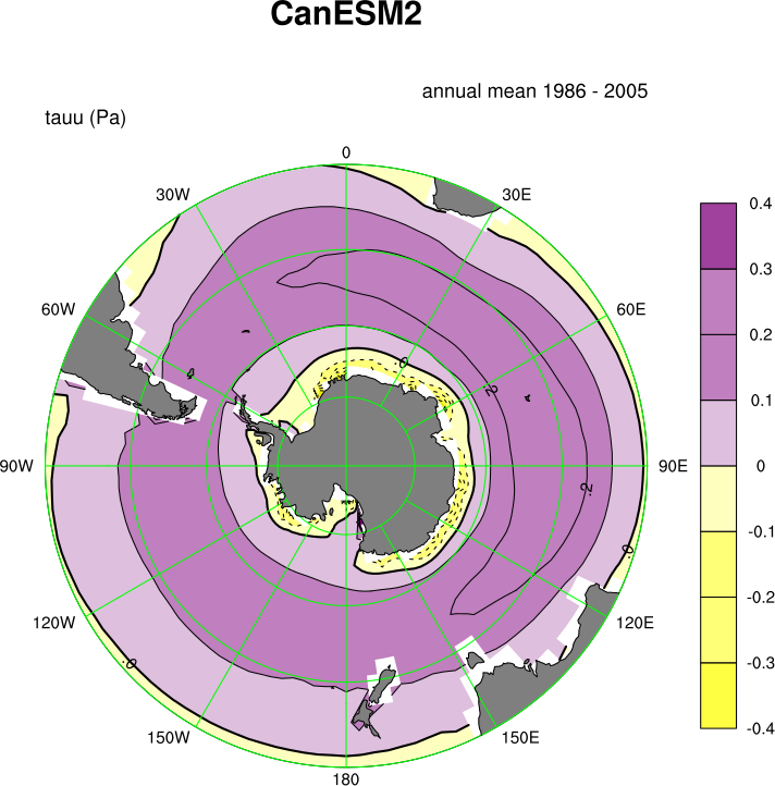
Fig. 181 Figure 1: Annual-mean zonal wind stress (tauu - N/m2) with eastward wind stress as positive plotted as a polar contour map.
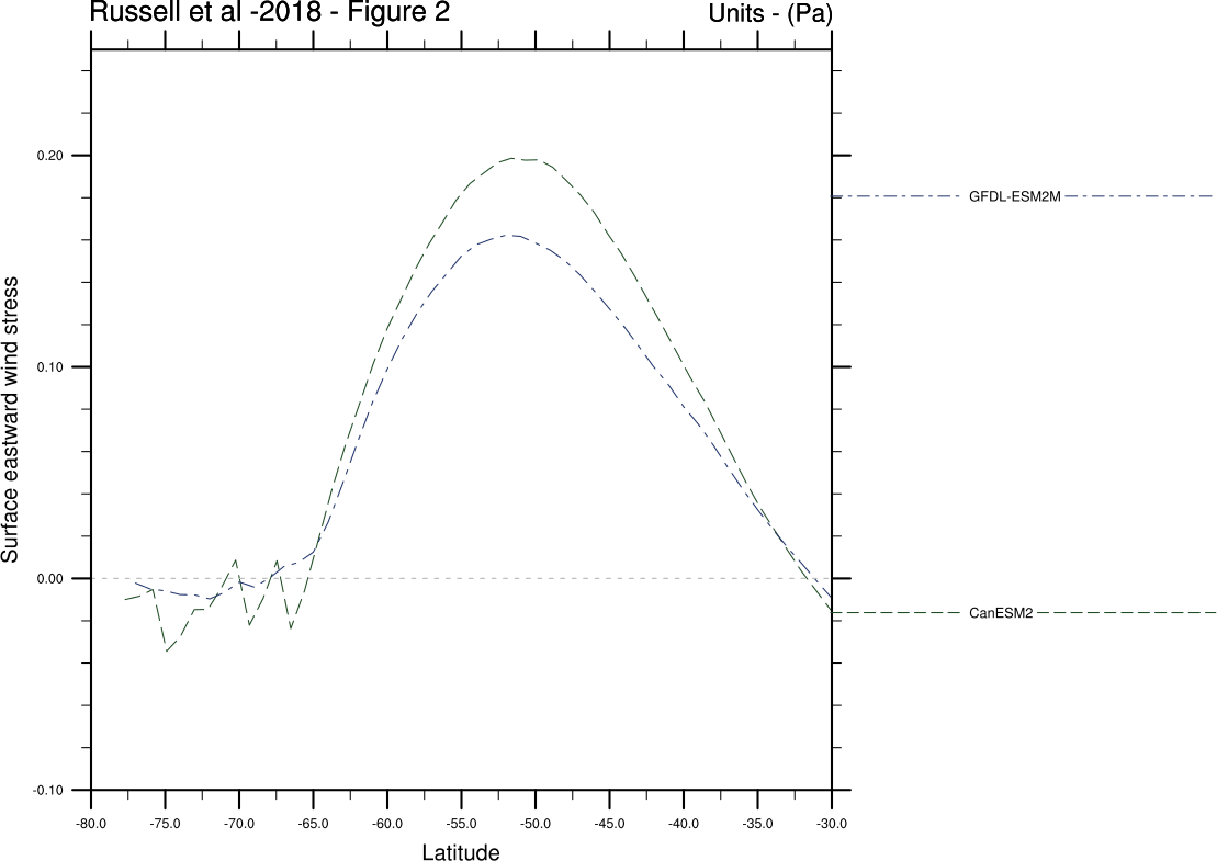
Fig. 182 Figure 2: The zonal and annual means of the zonal wind stress (N/m2) plotted in a line plot.
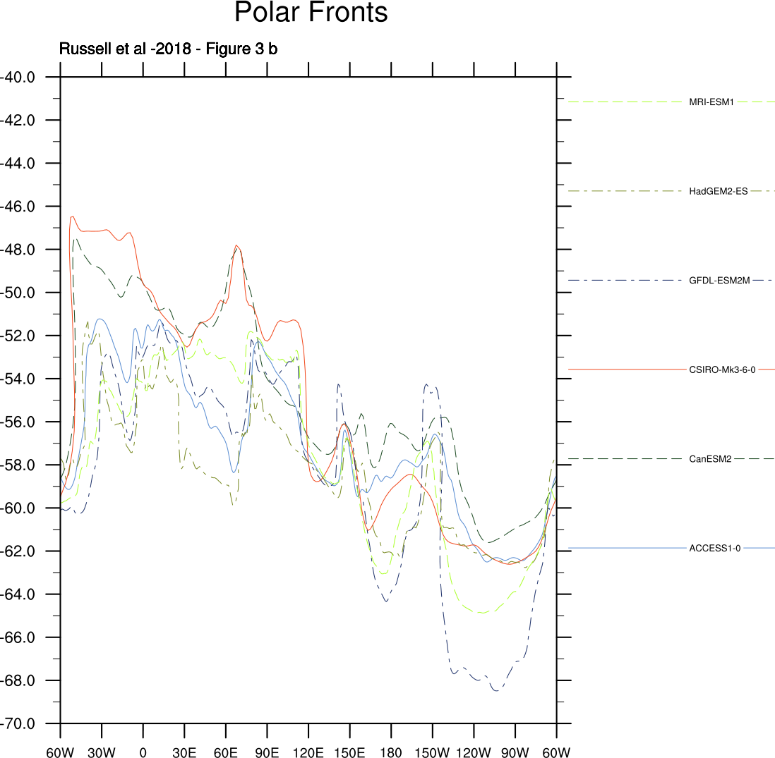
Fig. 183 Figure 3a: The latitudinal position of Subantarctic Front using definitions from Orsi et al (1995).
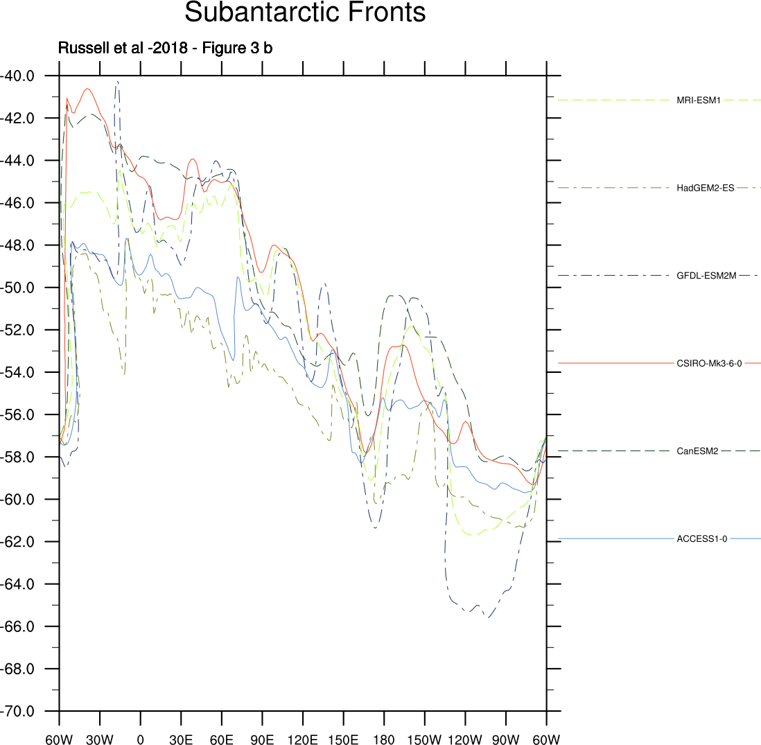
Fig. 184 Figure 3b: The latitudinal position of Polar Front using definitions from Orsi et al (1995).
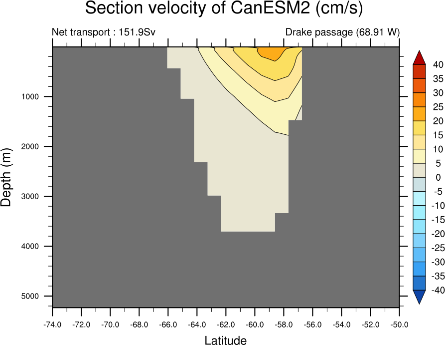
Fig. 185 Figure 4: Time averaged zonal velocity through Drake Passage (at 69W, in cm/s, eastward is positive). The total transport by the ACC is calculated if volcello file is available.
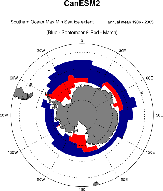
Fig. 186 Figure 5: Mean extent of sea ice for September(max) in blue and February(min) in red plotted as polar contour map.
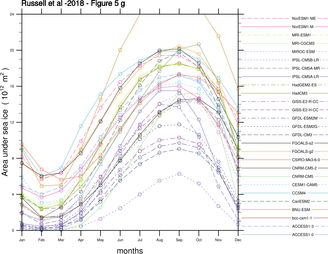
Fig. 187 Figure 5g: Annual cycle of sea ice area in southern ocean as a line plot (monthly climatology).
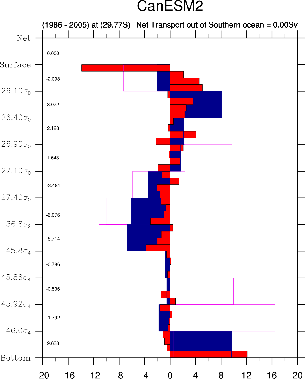
Fig. 188 Figure 6a: Density layer based volume transport (in Sv) across 30S based on the layer definitions in Talley (2008).
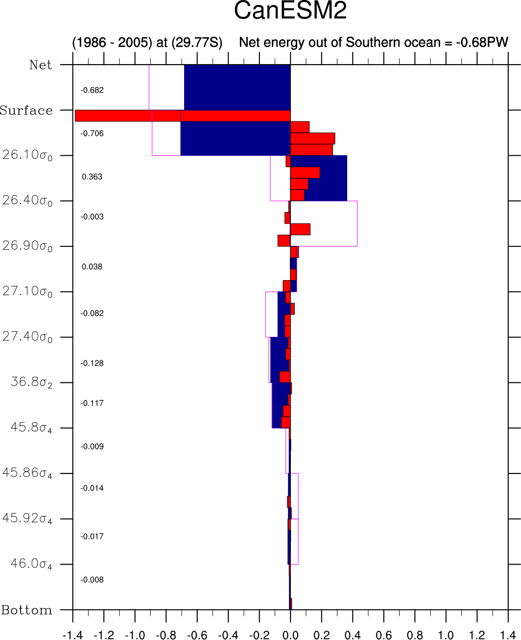
Fig. 189 Figure 6b: Density layer based heat transport(in PW) across 30S based on the layer definitions in Talley (2008).
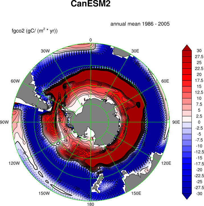
Fig. 190 Figure 7: Annual mean CO2 flux (sea to air, gC/(yr * m2), positive (red) is out of the ocean) as a polar contour map.
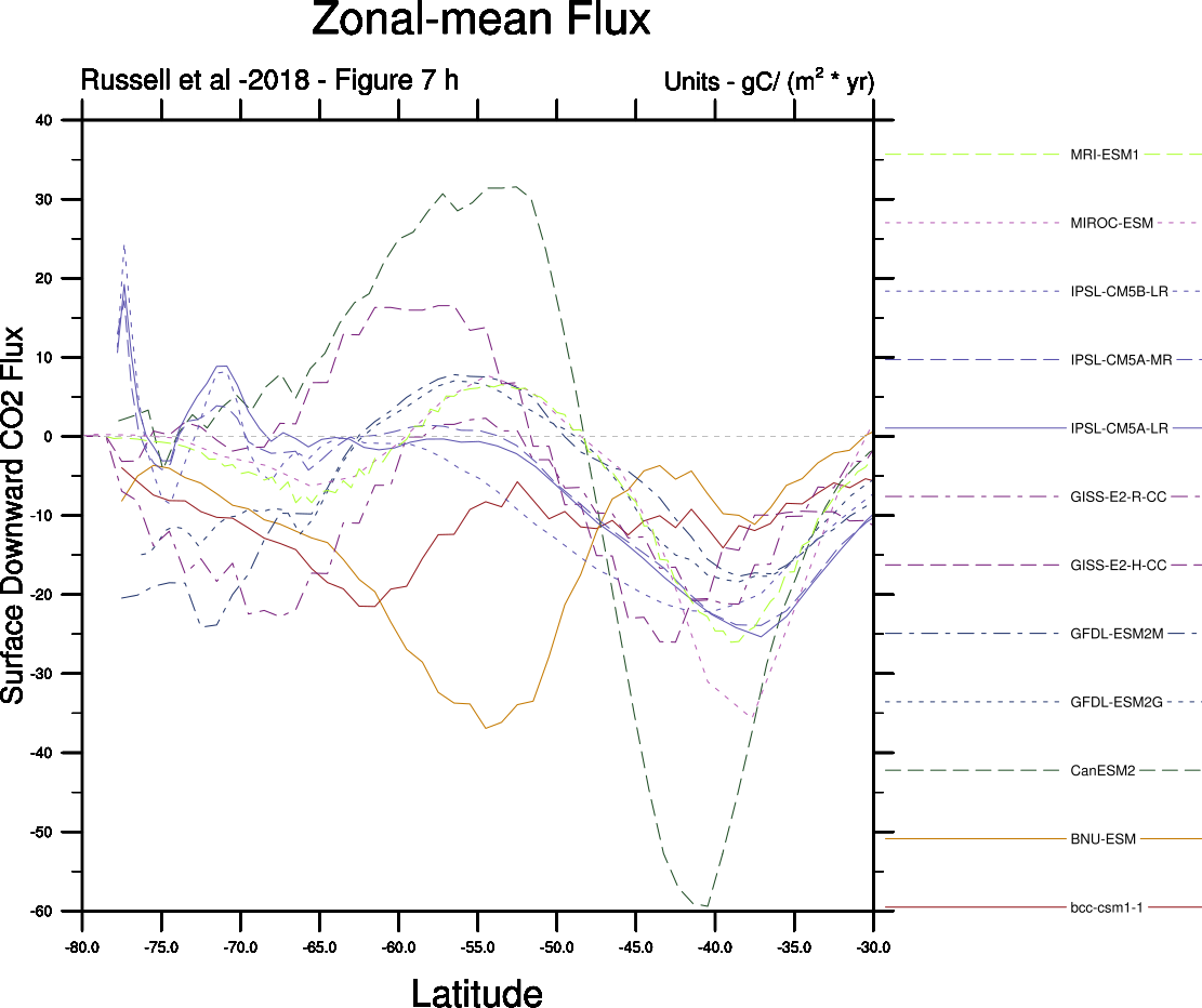
Fig. 191 Figure 7h: the time and zonal mean flux of CO2 in gC/(yr * m2) plotted as a line plot.
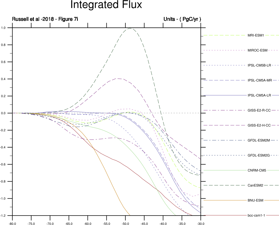
Fig. 192 Figure 7i is the cumulative integral of the net CO2 flux from 90S to 30S (in PgC/yr) plotted as a line plot.
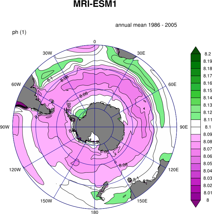
Fig. 193 Figure 8: Annual-mean surface pH plotted as a polar contour map.
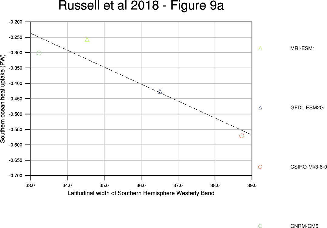
Fig. 194 Figure 9a: Scatter plot of the width of the Southern Hemisphere westerly wind band (in degrees of latitude) against the annual-mean integrated heat uptake south of 30S (in PW—negative uptake is heat lost from the ocean) along with the best fit line.
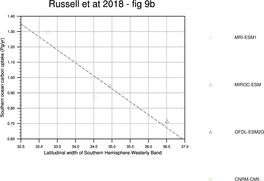
Fig. 195 Figure 9b: Scatter plot of the width of the Southern Hemisphere westerly wind band (in degrees of latitude) against the annual-mean integrated carbon uptake south of 30S (in Pg C/yr), along with the best fit line.
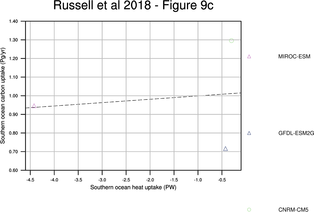
Fig. 196 Figure 9c: Scatter plot of the net heat uptake south of 30S (in PW) against the annual-mean integrated carbon uptake south of 30S (in Pg C/yr), along with the best fit line.