Ocean diagnostics
Overview
These recipes are used for evaluating the marine component of models of the earth system. Using these recipes, it should be possible to evaluate both the physical models and biogeochemistry models. All these recipes use the ocean diagnostics package.
The ocean diagnostics package contains several diagnostics which produce figures and statistical information of models of the ocean. The datasets have been pre-processed by ESMValTool, based on recipes in the recipes directory. Most of the diagnostics produce two or less types of figure, and several diagnostics are called by multiple recipes.
Each diagnostic script expects a metadata file, automatically generated by ESMValTool, and one or more pre-processed dataset. These are passed to the diagnostic by ESMValTool in the settings.yml and metadata.yml files.
The ocean diagnostics toolkit can not figure out how to plot data by itself. The current version requires the recipe to produce the correct pre-processed data for each diagnostic script. ie: to produce a time series plot, the preprocessor must produce a time-dimensional dataset.
While these tools were built to evaluate the ocean component models, they also can be used to produce figures for other domains. However, there are some ocean specific elements, such as the z-direction being positive and reversed, and some of the map plots have the continents coloured in by default.
As elsewhere, both the model and observational datasets need to be compliant with the CMOR data.
Available recipes
recipe_ocean_amoc.yml
The recipe_ocean_amoc.yml is an recipe that produces figures describing the Atlantic Meridional Overturning Circulation (AMOC) and the drake passage current.
The recipes produces time series of the AMOC at 26 north and the drake passage current.
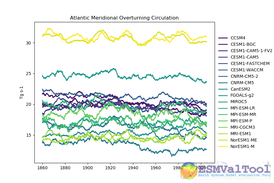
This figure shows the multi model comparison of the AMOC from several CMIP5 historical simulations, with a 6 year moving average (3 years either side of the central value). A similar figure is produced for each individual model, and for the Drake Passage current.
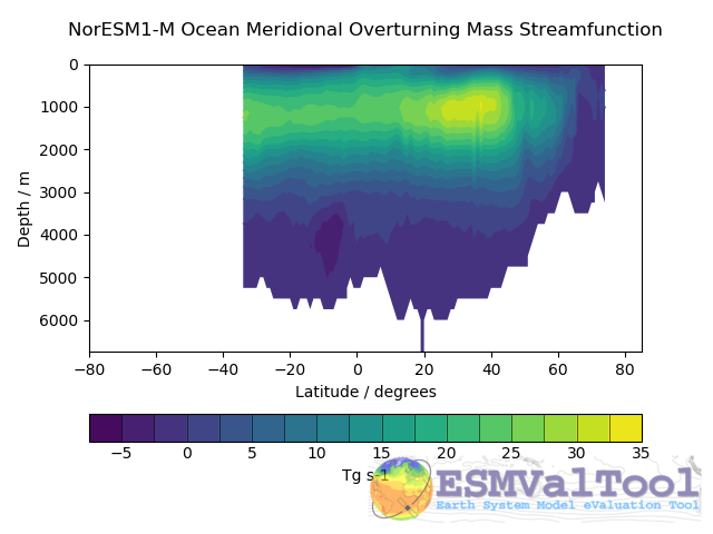
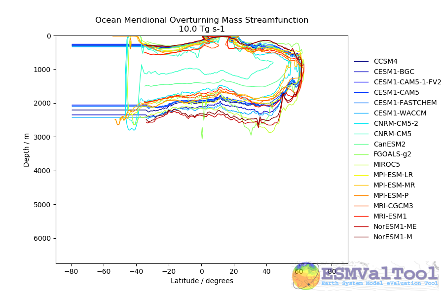
This recipe also produces a contour transect and a coloured transect plot showing the Atlantic stream function for each individual model, and a multi-model contour is also produced:
recipe_ocean_example.yml
The recipe_ocean_example.yml is an example recipe which shows several examples of how to manipulate marine model data using the ocean diagnostics tools.
While several of the diagnostics here have specific uses in evaluating models, it is meant to be a catch-all recipe demonstrating many different ways to evaluate models.
All example calculations are performed using the ocean temperature in a three dimensional field (thetao), or at the surface (tos). This recipe demonstrates the use of a range of preprocessors in a marine context, and also shows many of the standard model-only diagnostics (no observational component is included.)
This recipe includes examples of how to manipulate both 2D and 3D fields to produce:
Time series:
Global surface area weighted mean time series
Volume weighted average time series within a specific depth range
Area weighted average time series at a specific depth
Area weighted average time series at a specific depth in a specific region.
Global volume weighted average time series
Regional volume weighted average time series
Maps:
Global surface map (from 2D ad 3D initial fields)
Global surface map using re-gridding to a regular grid
Global map using re-gridding to a regular grid at a specific depth level
Regional map using re-gridding to a regular grid at a specific depth level
Transects:
Produce various transect figure showing a re-gridded transect plot, and multi model comparisons
Profile:
Produce a Global area-weighted depth profile figure
Produce a regional area-weighted depth profile figure
All the these fields can be expanded using a
recipe_ocean_bgc.yml
The recipe_ocean_bgc.yml is an example recipe which shows a several simple examples of how to manipulate marine biogeochemical model data.
This recipe includes the following fields:
Global total volume-weighted average time series:
temperature, salinity, nitrate, oxygen, silicate (vs WOA data) *
chlorophyll, iron, total alkalinity (no observations)
Surface area-weighted average time series:
temperature, salinity, nitrate, oxygen, silicate (vs WOA data) *
fgco2 (global total), integrated primary production, chlorophyll, iron, total alkalinity (no observations)
Scalar fields time series:
mfo (including stuff like drake passage)
Profiles:
temperature, salinity, nitrate, oxygen, silicate (vs WOA data) *
chlorophyll, iron, total alkalinity (no observations)
Maps + contours:
temperature, salinity, nitrate, oxygen, silicate (vs WOA data) *
chlorophyll, iron, total alkalinity (no observations)
Transects + contours:
temperature, salinity, nitrate, oxygen, silicate (vs WOA data) *
chlorophyll, iron, no observations)
* Note that Phosphate is also available as a WOA diagnostic, but I haven’t included it as HadGEM2-ES doesn’t include a phosphate field.
This recipe uses the World Ocean Atlas data, which can be downloaded from: https://www.ncei.noaa.gov/products/world-ocean-atlas (last access 02/08/2021)
Instructions: Select the “All fields data links (1° grid)” netCDF file, which contain all fields.
recipe_ocean_quadmap.yml
The recipe_ocean_quadmap.yml is an example recipe showing the diagnostic_maps_quad.py diagnostic. This diagnostic produces an image showing four maps. Each of these four maps show latitude vs longitude and the cube value is used as the colour scale. The four plots are:
model1 |
model 1 minus model2 |
model2 minus obs |
model1 minus obs |
These figures are also known as Model vs Model vs Obs plots.
The figure produced by this recipe compares two versions of the HadGEM2 model against ATSR sea surface temperature:
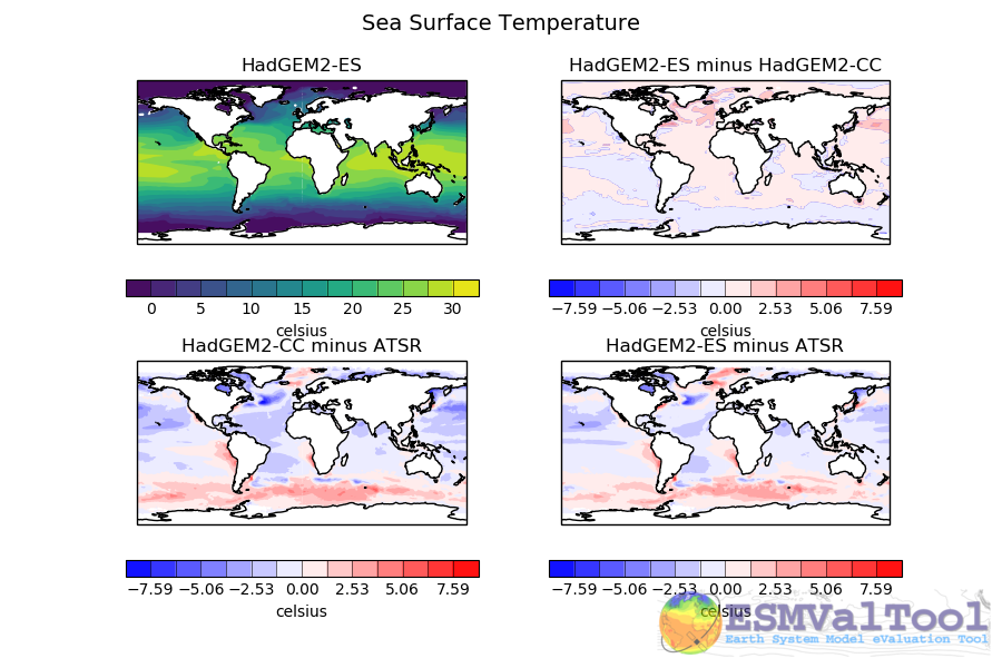
This kind of figure can be very useful when developing a model, as it allows model developers to quickly see the impact of recent changes to the model.
recipe_ocean_ice_extent.yml
The recipe_ocean_ice_extent.yml recipe produces several metrics describing the behaviour of sea ice in a model, or in multiple models.
This recipe has four preprocessors, a combinatorial combination of
Regions: Northern or Southern Hemisphere
Seasons: December-January-February or June-July-August
Once these seasonal hemispherical fractional ice cover is processed, the resulting cube is passed ‘as is’ to the diagnostic_seaice.py diagnostic.
This diagnostic produces the plots:
Polar Stereographic projection Extent plots of individual models years.
Polar Stereographic projection maps of the ice cover and ice extent for individual models.
A time series of Polar Stereographic projection Extent plots - see below.
Time series plots of the total ice area and the total ice extent.
The following image shows an example of the sea ice extent plot, showing the Summer Northern hemisphere ice extent for the HadGEM2-CC model, in the historical scenario.
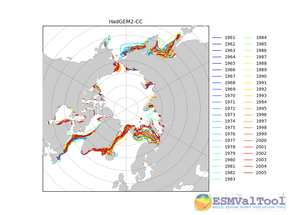
The sea ice diagnostic is unlike the other diagnostics in the ocean diagnostics
toolkit. The other tools are build to be generic plotting tools which
work with any field (ie diagnostic_timeseries.py works fine for Temperature,
Chlorophyll, or any other field. On the other hand, the
sea ice diagnostic is the only tool that performs a field specific evaluation.
The diagnostic_seaice.py diagnostic is more fully described below.
recipe_ocean_multimap.yml
The recipe_ocean_multimap.yml is an example recipe showing the diagnostic_maps_multimodel.py diagnostic. This diagnostic produces an image showing Model vs Observations maps or only Model fields when observational data are not provided. Each map shows latitude vs longitude fields and user defined values are used to set the colour scale. Plot layout can be modified by modifying the layout_rowcol argument.
The figure produced by this recipe compares the ocean surface CO2 fluxes for 16 different CMIP5 model against Landschuetzer2016 observations.
The diagnostic_maps_multimodel.py diagnostic is documented below.
Available diagnostics
Diagnostics are stored in the diag_scripts directory: ocean.
The following python modules are included in the ocean diagnostics package. Each module is described in more detail both below and inside the module.
diagnostic_maps.py
diagnostic_maps_quad.py
diagnostic_model_vs_obs.py
diagnostic_profiles.py
diagnostic_seaice.py
diagnostic_timeseries.py
diagnostic_tools.py
diagnostic_transects.py
diagnostic_maps_multimodel.py
diagnostic_maps.py
The diagnostic_maps.py produces a spatial map from a NetCDF. It requires the input netCDF to have the following dimensions. Either:
A two dimensional file: latitude, longitude.
A three dimensional file: depth, latitude, longitude.
In the case of a 3D netCDF file, this diagnostic produces a map for EVERY layer. For this reason, we recommend extracting a small number of specific layers in the preprocessor, using the extract_layer preprocessor.
This script can not process NetCDFs with multiple time steps. Please use the climate_statistics preprocessor to collapse the time dimension.
This diagnostic also includes the optional arguments, threshold and thresholds.
threshold: a single float.
thresholds: a list of floats.
Only one of these arguments should be provided at a time. These two arguments produce a second kind of diagnostic map plot: a contour map showing the spatial distribution of the threshold value, for each dataset. Alternatively, if the thresholds argument is used instead of threshold, the single-dataset contour map shows the contours of all the values in the thresholds list.
If multiple datasets are provided, in addition to the single dataset contour, a multi-dataset contour map is also produced for each value in the thresholds list.
Some appropriate preprocessors for this diagnostic would be:
For a Global 2D field:
prep_map_1:
  climate_statistics:
For a regional 2D field:
prep_map_2:
    extract_region:
      start_longitude: -80.
      end_longitude: 30.
      start_latitude: -80.
      end_latitude: 80.
climate_statistics:
  operator: mean
For a Global 3D field at the surface and 10m depth:
  prep_map_3:
    custom_order: true
    extract_levels:
      levels: [0., 10.]
      scheme: linear_horizontal_extrapolate_vertical
climate_statistics:
  operator: mean
For a multi-model comparison mean of 2D global fields including contour thresholds.
  prep_map_4:
    custom_order: true
climate_statistics:
  operator: mean
    regrid:
      target_grid: 1x1
      scheme: linear
And this also requires the threshold key in the diagnostic:
diagnostic_map:
  variables:
    tos: # Temperature ocean surface
      preprocessor: prep_map_4
      field: TO2M
  scripts:
    Ocean_regrid_map:
      script: ocean/diagnostic_maps.py
      thresholds: [5, 10, 15, 20]
diagnostic_maps_quad.py
The diagnostic_maps_quad.py diagnostic produces an image showing four maps. Each of these four maps show latitude vs longitude and the cube value is used as the colour scale. The four plots are:
model1 |
model 1 minus model2 |
model2 minus obs |
model1 minus obs |
These figures are also known as Model vs Model vs Obs plots.
This diagnostic assumes that the preprocessors do the bulk of the hard work, and that the cubes received by this diagnostic (via the settings.yml and metadata.yml files) have no time component, a small number of depth layers, and a latitude and longitude coordinates.
An appropriate preprocessor for a 2D field would be:
prep_quad_map:
climate_statistics:
    operator: mean
and an example of an appropriate diagnostic section of the recipe would be:
diag_map_1:
  variables:
    tos: # Temperature ocean surface
      preprocessor: prep_quad_map
      field: TO2Ms
      mip: Omon
  additional_datasets:
#        filename: tos_ATSR_L3_ARC-v1.1.1_199701-201112.nc
#        download from: https://datashare.is.ed.ac.uk/handle/10283/536
    - {dataset: ATSR,  project: obs4MIPs,  level: L3,  version: ARC-v1.1.1,  start_year: 2001,  end_year: 2003, tier: 3}
  scripts:
    Global_Ocean_map:
      script: ocean/diagnostic_maps_quad.py
      control_model: {dataset: HadGEM2-CC, project: CMIP5, mip: Omon, exp: historical, ensemble: r1i1p1}
      exper_model: {dataset: HadGEM2-ES, project: CMIP5, mip: Omon, exp: historical, ensemble: r1i1p1}
      observational_dataset: {dataset: ATSR, project: obs4MIPs,}
Note that the details about the control model, the experiment models and the observational dataset are all provided in the script section of the recipe.
diagnostic_model_vs_obs.py
The diagnostic_model_vs_obs.py diagnostic makes model vs observations maps and scatter plots. The map plots shows four latitude vs longitude maps:
Model |
Observations |
Model minus Observations |
Model over Observations |
Note that this diagnostic assumes that the preprocessors do the bulk of the hard work, and that the cube received by this diagnostic (via the settings.yml and metadata.yml files) has no time component, a small number of depth layers, and a latitude and longitude coordinates.
This diagnostic also includes the optional arguments, maps_range and diff_range to manually define plot ranges. Both arguments are a list of two floats to set plot range minimun and maximum values respectively for Model and Observations maps (Top panels) and for the Model minus Observations panel (bottom left). Note that if input data have negative values the Model over Observations map (bottom right) is not produced.
The scatter plots plot the matched model coordinate on the x axis, and the observational dataset on the y coordinate, then performs a linear regression of those data and plots the line of best fit on the plot. The parameters of the fit are also shown on the figure.
An appropriate preprocessor for a 3D+time field would be:
preprocessors:
  prep_map:
    extract_levels:
      levels:  [100., ]
      scheme: linear_extrap
climate_statistics:
  operator: mean
    regrid:
      target_grid: 1x1
      scheme: linear
diagnostic_maps_multimodel.py
The diagnostic_maps_multimodel.py diagnostic makes model(s) vs observations maps and if data are not provided it draws only model field.
It is always nessary to define the overall layout trough the argument layout_rowcol, which is a list of two integers indicating respectively the number of rows and columns to organize the plot. Observations has not be accounted in here as they are automatically added at the top of the figure.
This diagnostic also includes the optional arguments, maps_range and diff_range to manually define plot ranges. Both arguments are a list of two floats to set plot range minimun and maximum values respectively for variable data and the Model minus Observations range.
Note that this diagnostic assumes that the preprocessors do the bulk of the hard work, and that the cube received by this diagnostic (via the settings.yml and metadata.yml files) has no time component, a small number of depth layers, and a latitude and longitude coordinates.
An appropriate preprocessor for a 3D+time field would be:
preprocessors:
  prep_map:
    extract_levels:
      levels:  [100., ]
      scheme: linear_extrap
climate_statistics:
  operator: mean
    regrid:
      target_grid: 1x1
      scheme: linear
diagnostic_profiles.py
The diagnostic_profiles.py diagnostic produces images of the profile over time from a cube. These plots show cube value (ie temperature) on the x-axis, and depth/height on the y axis. The colour scale is the annual mean of the cube data. Note that this diagnostic assumes that the preprocessors do the bulk of the hard work, and that the cube received by this diagnostic (via the settings.yml and metadata.yml files) has a time component, and depth component, but no latitude or longitude coordinates.
An appropriate preprocessor for a 3D+time field would be:
preprocessors:
  prep_profile:
    extract_volume:
      long1: 0.
      long2:  20.
      lat1:  -30.
      lat2:  30.
      z_min: 0.
      z_max: 3000.
    area_statistics:
      operator: mean
diagnostic_timeseries.py
The diagnostic_timeseries.py diagnostic produces images of the time development of a metric from a cube. These plots show time on the x-axis and cube value (ie temperature) on the y-axis.
Two types of plots are produced: individual model timeseries plots and multi model time series plots. The individual plots show the results from a single cube, even if this cube is a multi-model mean made by the multimodel preprocessor.
The multi model time series plots show several models on the same axes, where each model is represented by a different line colour. The line colours are determined by the number of models, their alphabetical order and the jet colour scale. Observational datasets and multimodel means are shown as black lines.
This diagnostic assumes that the preprocessors do the bulk of the work, and that the cube received by this diagnostic (via the settings.yml and metadata.yml files) is time-dimensional cube. This means that the pre-processed netcdf has a time component, no depth component, and no latitude or longitude coordinates.
Some appropriate preprocessors would be :
For a global area-weighted average 2D field:
area_statistics:
  operator: mean
For a global volume-weighted average 3D field:
volume_statistics:
  operator: mean
For a global area-weighted surface of a 3D field:
extract_levels:
  levels: [0., ]
  scheme: linear_horizontal_extrapolate_vertical
area_statistics:
  operator: mean
An example of the multi-model time series plots can seen here:
diagnostic_transects.py
The diagnostic_transects.py diagnostic produces images of a transect, typically along a constant latitude or longitude.
These plots show 2D plots with either latitude or longitude along the x-axis, depth along the y-axis and and the cube value is used as the colour scale.
This diagnostic assumes that the preprocessors do the bulk of the hard work, and that the cube received by this diagnostic (via the settings.yml and metadata.yml files) has no time component, and one of the latitude or longitude coordinates has been reduced to a single value.
An appropriate preprocessor for a 3D+time field would be:
climate_statistics:
  operator: mean
extract_slice:
  latitude: [-50.,50.]
  longitude: 332.
Here is an example of the transect figure:
.. centered::
And here is an example of the multi-model transect contour figure:
diagnostic_seaice.py
The diagnostic_seaice.py diagnostic is unique in this module, as it produces several different kinds of images, including time series, maps, and contours. It is a good example of a diagnostic where the preprocessor does very little work, and the diagnostic does a lot of the hard work.
This was done purposely, firstly to demonstrate the flexibility of ESMValTool, and secondly because Sea Ice is a unique field where several Metrics can be calculated from the sea ice cover fraction.
The recipe Associated with with diagnostic is the recipe_SeaIceExtent.yml. This recipe contains 4 preprocessors which all perform approximately the same calculation. All four preprocessors extract a season: - December, January and February (DJF) - June, July and August (JJA) and they also extract either the North or South hemisphere. The four preprocessors are combinations of DJF or JJA and North or South hemisphere.
One of the four preprocessors is North Hemisphere Winter ice extent:
timeseries_NHW_ice_extent: # North Hemisphere Winter ice_extent
  custom_order: true
  extract_time: &time_anchor # declare time here.
      start_year: 1960
      start_month: 12
      start_day: 1
      end_year: 2005
      end_month: 9
      end_day: 31
  extract_season:
    season: DJF
  extract_region:
    start_longitude: -180.
    end_longitude: 180.
    start_latitude: 0.
    end_latitude: 90.
Note that the default settings for ESMValTool assume that the year starts on the first of January. This causes a problem for this preprocessor, as the first DJF season would not include the first Month, December, and the final would not include both January and February. For this reason, we also add the extract_time preprocessor.
This preprocessor group produces a 2D field with a time component, allowing the diagnostic to investigate the time development of the sea ice extend.
The diagnostic section of the recipe should look like this:
diag_ice_NHW:
  description: North Hemisphere Winter Sea Ice diagnostics
  variables:
    sic: # surface ice cover
      preprocessor: timeseries_NHW_ice_extent
      field: TO2M
      mip: OImon
  scripts:
    Global_seaice_timeseries:
      script: ocean/diagnostic_seaice.py
      threshold: 15.
Note the the threshold here is 15%, which is the standard cut of for the ice extent.
The sea ice diagnostic script produces three kinds of plots, using the methods:
make_map_extent_plots: extent maps plots of individual models using a Polar Stereographic project.
make_map_plots: maps plots of individual models using a Polar Stereographic project.
make_ts_plots: time series plots of individual models
There are no multi model comparisons included here (yet).
diagnostic_tools.py
The diagnostic_tools.py is a module that contains several python tools used by the ocean diagnostics tools.
These tools are:
folder: produces a directory at the path provided and returns a string.
get_input_files: loads a dictionary from the input files in the metadata.yml.
bgc_units: converts to sensible units where appropriate (ie Celsius, mmol/m3)
timecoord_to_float: Converts time series to decimal time ie: Midnight on January 1st 1970 is 1970.0
add_legend_outside_right: a plotting tool, which adds a legend outside the axes.
get_image_format: loads the image format, as defined in the global user config.yml.
get_image_path: creates a path for an image output.
make_cube_layer_dict: makes a dictionary for several layers of a cube.
We just show a simple description here, each individual function is more fully documented in the diagnostic_tools.py module.
A note on the auxiliary data directory
Some of these diagnostic scripts may not function on machines with no access to the internet, as cartopy may try to download the shape files. The solution to this issue is the put the relevant cartopy shapefiles in a directory which is visible to esmvaltool, then link that path to ESMValTool via the auxiliary_data_dir variable in your config-user.yml file.
The cartopy masking files can be downloaded from: https://www.naturalearthdata.com/downloads/
In these recipes, cartopy uses the 1:10, physical coastlines and land files:
110m_coastline.dbf
110m_coastline.shp
110m_coastline.shx
110m_land.dbf
110m_land.shp
110m_land.shx
Associated Observational datasets
The following observations datasets are used by these recipes:
World Ocean ATLAS
These data can be downloaded from: https://www.nodc.noaa.gov/OC5/woa13/woa13data.html (last access 10/25/2018) Select the “All fields data links (1° grid)” netCDF file, which contain all fields.
- The following WOA datasets are used by the ocean diagnostics:
Temperature
Salinity
Nitrate
Phosphate
Silicate
Dissolved Oxygen
These files need to be reformatted using the esmvaltool data format WOA command.
Landschuetzer 2016
These data can be downloaded from: https://www.nodc.noaa.gov/archive/arc0105/0160558/3.3/data/0-data/spco2_1982-2015_MPI_SOM-FFN_v2016.nc (last access 09/20/2022)
- The following variables are used by the ocean diagnostics:
fgco2, Surface Downward Flux of Total CO2
spco2, Surface Aqueous Partial Pressure of CO2
dpco2, Delta CO2 Partial Pressure
The file needs to be reformatted using the esmvaltool data format Landschuetzer2016 command.