Turnover time of carbon over land ecosystems

Overview

This recipe evaluates the turnover time of carbon over land ecosystems (tau_ctotal) based on the analysis of Carvalhais et al. (2014). In summary, it provides an overview on:

• Comparisons of global distributions of tau_ctotal from all models against observation and other models

• Variation of tau_ctotal across latitude (zonal distributions)

• Variation of association of tau_ctotal and climate across latitude (zonal correlations)

• metrics of global tau_ctotal and correlations

Calculation of turnover time

First, the total carbon content of land ecosystems is calculated as,

\[ctotal = cSoil + cVeg\]

where \(cSoil\) and \(cVeg\) are the carbon contents in soil and vegetation. Note that this is not fully consistent with `Carvalhais et al. (2014)`_, in which `ctotal` includes all carbon storages that respire to the atmosphere. Due to inconsistency across models, it resulted in having different carbon storage components in calculation of ctotal for different models.

The turnover time of carbon is then calculated as,

\[\tau_{ctotal} = \frac{ctotal}{gpp}\]

where ctotal and gpp are temporal means of total carbon content and gross primary productivity, respectively. The equation is valid for steady state, and is only applicable when both ctotal and gpp are long-term averages. Therefore, the recipe should always include the mean operator of climate_statistics in preprocessor.

Available recipes and diagnostics

Recipes are stored in recipes/

• recipe_carvalhais14nat.yml

Diagnostics are stored in diag_scripts/

• land_carbon_cycle/diag_global_turnover.py

• land_carbon_cycle/diag_zonal_turnover.py

• land_carbon_cycle/diag_zonal_correlation.py

User settings in recipe

Observation-related details

The settings needed for loading the observational dataset in all diagnostics are provided in the recipe through obs_info within obs_details section.

• obs_data_subdir: subdirectory of auxiliary_data_dir (set in config-user file) where observation data are stored {e.g., data_ESMValTool_Carvalhais2014}.

• source_label: source data label {‘Carvalhais2014’}.

• variant_label: variant of the observation {‘BE’} for best estimate.

• grid_label: label denoting the spatial grid specification {‘gn’}.

• frequency: temporal frequency of the observation data {‘fx’}

The observation data file used in the recipe should be changed through the fields above, as these are used to generate observation file name and locations. For details, see Observations section.

Preprocessor

• climate_statistics: {mean} - calculate the mean over full time period.

• regrid: {nearest} - nearest neighbor regridding to the selected observation resolution.

• mask_landsea: {sea} - mask out all the data points from sea.

• multi_model_statistics: {median} - calculate and include the multimodel median.

Script land_carbon_cycle/diag_global_turnover.py

• Required settings:

  • obs_variable: {str} list of the variable(s) to be read from the observation files

• Optional settings:

  • ax_fs: {float, 7.1} - fontsize in the figure.

  • fill_value: {float, nan} - fill value to be used in analysis and plotting.

  • x0: {float, 0.02} - X - coordinate of the left edge of the figure.

  • y0: {float, 1.0} Y - coordinate of the upper edge of the figure.

  • wp: {float, 1 / number of models} - width of each map.

  • hp: {float, = wp} - height of each map.

  • xsp: {float, 0} - spacing betweeen maps in X - direction.

  • ysp: {float, -0.03} - spacing between maps in Y -direction. Negative to reduce the spacing below default.

  • aspect_map: {float, 0.5} - aspect of the maps.

  • xsp_sca: {float, wp / 1.5} - spacing between the scatter plots in X - direction.

  • ysp_sca: {float, hp / 1.5} - spacing between the scatter plots in Y - direction.

  • hcolo: {float, 0.0123} - height (thickness for horizontal orientation) of the colorbar .

  • wcolo: {float, 0.25} - width (length) of the colorbar.

  • cb_off_y: {float, 0.06158} - distance of colorbar from top of the maps.

  • x_colo_d: {float, 0.02} - X - coordinate of the colorbar for maps along the diagonal (left).

  • x_colo_r: {float, 0.76} - Y - coordinate of the colorbar for ratio maps above the diagonal (right).

  • y_colo_single: {float, 0.1086} - Y-coordinate of the colorbar in the maps per model (separate figures).

  • correlation_method: {str, spearman | pearson} - correlation method to be used while calculating the correlation displayed in the scatter plots.

  • tx_y_corr: {float, 1.075} - Y - coordinate of the inset text of correlation.

  • valrange_sc: {tuple, (2, 256)} - range of turnover times in X - and Y - axes of scatter plots.

  • obs_global: {float, 23} - global turnover time, provided as additional info for map of the observation. For models, they are calculated within the diagnostic.

  • gpp_threshold: {float, 0.01} - The threshold of gpp in kg m^{-2} yr^{-1} below which the grid cells are masked.

Script land_carbon_cycle/diag_zonal_turnover.py

• Required settings:

  • obs_variable: {str} list of the variable(s) to be read from the observation files

• Optional settings:

  • ax_fs: {float, 7.1} - fontsize in the figure.

  • fill_value: {float, nan} - fill value to be used in analysis and plotting.

  • valrange_x: {tuple, (2, 1000)} - range of turnover values in the X - axis.

  • valrange_y: {tuple, (-70, 90)} - range of latitudes in the Y - axis.

  • bandsize: {float, 9.5} - size of the latitudinal rolling window in degrees. One latitude row if set to None.

  • gpp_threshold: {float, 0.01} - The threshold of gpp in kg m^{-2} yr^{-1} below which the grid cells are masked.

Script land_carbon_cycle/diag_zonal_correlation.py

• Required settings:

  • obs_variable: {str} list of the variable(s) to be read from the observation files

• Optional settings:

  • ax_fs: {float, 7.1} - fontsize in the figure.

  • fill_value: {float, nan} - fill value to be used in analysis and plotting.

  • correlation_method: {str, pearson | spearman} - correlation method to be used while calculating the zonal correlation.

  • min_points_frac: {``float, 0.125} - minimum fraction of valid points within the latitudinal band for calculation of correlation.

  • valrange_x: {tuple, (-1, 1)} - range of correlation values in the X - axis.

  • valrange_y: {tuple, (-70, 90)} - range of latitudes in the Y - axis.

  • bandsize: {float, 9.5} - size of the latitudinal rolling window in degrees. One latitude row if set to None.

  • gpp_threshold: {float, 0.01} - The threshold of gpp in kg m^{-2} yr^{-1} below which the grid cells are masked.

Required Variables

• tas (atmos, monthly, longitude, latitude, time)

• pr (atmos, monthly, longitude, latitude, time)

• gpp (land, monthly, longitude, latitude, time)

• cVeg (land, monthly, longitude, latitude, time)

• cSoil (land, monthly, longitude, latitude, time)

Observations

The observations needed in the diagnostics are publicly available for download from the Data Portal of the Max Planck Institute for Biogeochemistry after registration.

Due to inherent dependence of the diagnostic on uncertainty estimates in observation, the data needed for each diagnostic script are processed at different spatial resolutions (as in Carvalhais et al., 2014), and provided in 11 different resolutions (see Table 1). Note that the uncertainties were estimated at the resolution of the selected models, and, thus, only the pre-processed observed data can be used with the recipe. It is not possible to use regridding functionalities of ESMValTool to regrid the observational data to other spatial resolutions, as the uncertainty estimates cannot be regridded.

Table 1. A summary of the observation datasets at different resolutions.

Reference	target_grid	grid_label*
Observation	0.5x0.5	gn
NorESM1-M	2.5x1.875	gr
bcc-csm1-1	2.812x2.813	gr1
CCSM4	1.25x0.937	gr2
CanESM2	2.812x2.813	gr3
GFDL-ESM2G	2.5x2.0	gr4
HadGEM2-ES	1.875x1.241	gr5
inmcm4	2.0x1.5	gr6
IPSL-CM5A-MR	2.5x1.259	gr7
MIROC-ESM	2.812x2.813	gr8
MPI-ESM-LR	1.875x1.875	gr9

* The grid_label is suffixed with z for data in zonal/latitude coordinates: the zonal turnover and zonal correlation.

To change the spatial resolution of the evaluation, change {grid_label} in obs_details and the corresponding {target_grid} in regrid preprocessor of the recipe.

At each spatial resolution, four data files are provided:

• tau_ctotal_fx_Carvalhais2014_BE_gn.nc - global data of tau_ctotal

• tau_ctotal_fx_Carvalhais2014_BE_gnz.nc - zonal data of tau_ctotal

• r_tau_ctotal_tas_fx_Carvalhais2014_BE_gnz.nc - zonal correlation of tau_ctotal and tas, controlled for pr

• r_tau_ctotal_pr_fx_Carvalhais2014_BE_gnz.nc - zonal correlation of tau_ctotal and pr, controlled for tas.

The data is produced in obs4MIPs standards, and provided in netCDF4 format. The filenames use the convention:

{variable}_{frequency}_{source_label}_{variant_label}_{grid_label}.nc

• {variable}: variable name, set in every diagnostic script as obs_variable

• {frequency}: temporal frequency of data, set from obs_details

• {source_label}: observational source, set from obs_details

• {variant_label}: observation variant, set from obs_details

• {grid_label}: temporal frequency of data, set from obs_details

Refer to the Obs4MIPs Data Specifications for details of the definitions above.

All data variables have additional variables ({variable}_5 and {variable}_95) in the same file. These variables are necessary for a successful execution of the diagnostics.

References

• Carvalhais, N., et al. (2014), Global covariation of carbon turnover times with climate in terrestrial ecosystems, Nature, 514(7521), 213-217, doi: 10.1038/nature13731.

Example plots

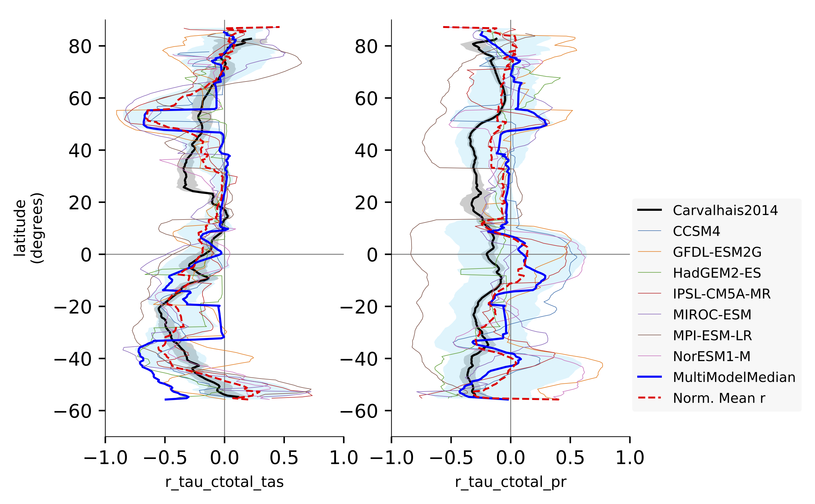
Fig. 137 Comparison of latitudinal (zonal) variations of pearson correlation between turnover time and climate: turnover time and precipitation, controlled for temperature (left) and vice-versa (right). Reproduces figures 2c and 2d in Carvalhais et al. (2014).

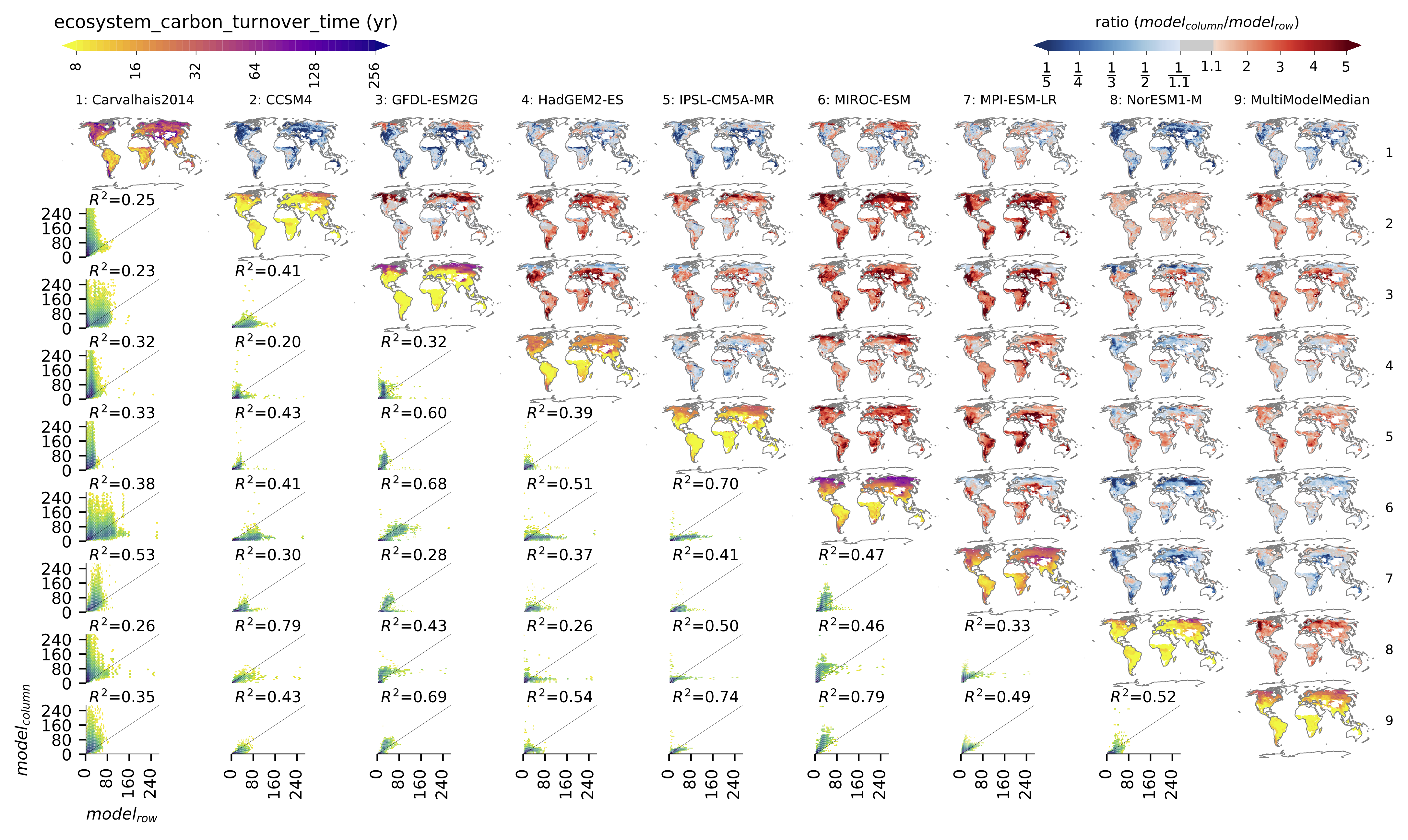
Fig. 138 Comparison of observation-based and modelled ecosystem carbon turnover time. Along the diagnonal, tau_ctotal are plotted, above the bias, and below density plots. The inset text in density plots indicate the correlation.

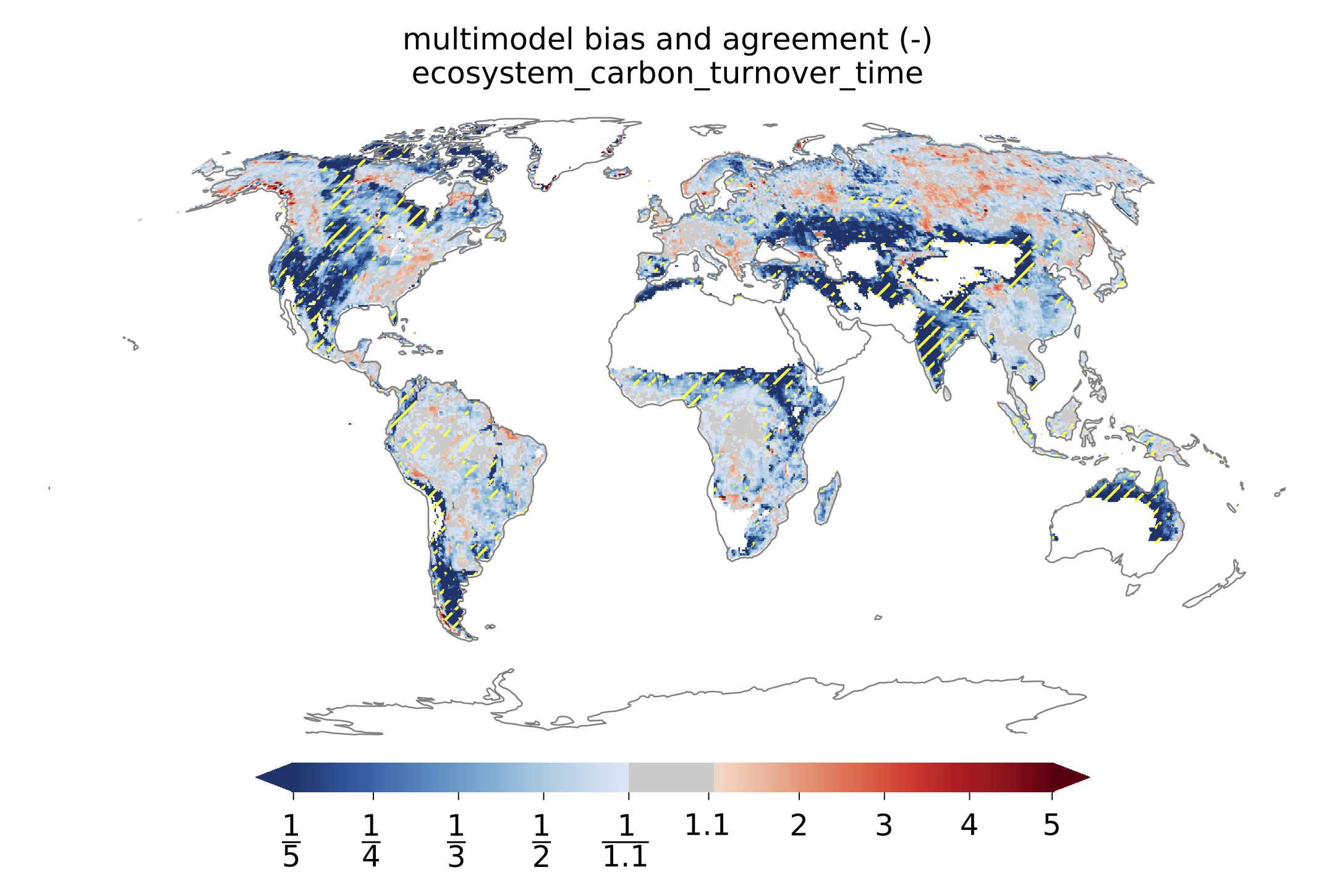
Fig. 139 Global distributions of multimodel bias and model agreement. Multimodel bias is calculated as the ratio of multimodel median turnover time and that from observation. Stippling indicates the regions where only less than one quarter of the models fall within the range of observational uncertainties (5^{th} and 95^{th} percentiles). Reproduces figure 3 in Carvalhais et al. (2014).

Fig. 140 Comparison of latitudinal (zonal) variations of observation-based and modelled ecosystem carbon turnover time. The zonal turnover time is calculated as the ratio of zonal ctotal and gpp. Reproduces figures 2a and 2b in Carvalhais et al. (2014).