Landcover diagnostics
Overview
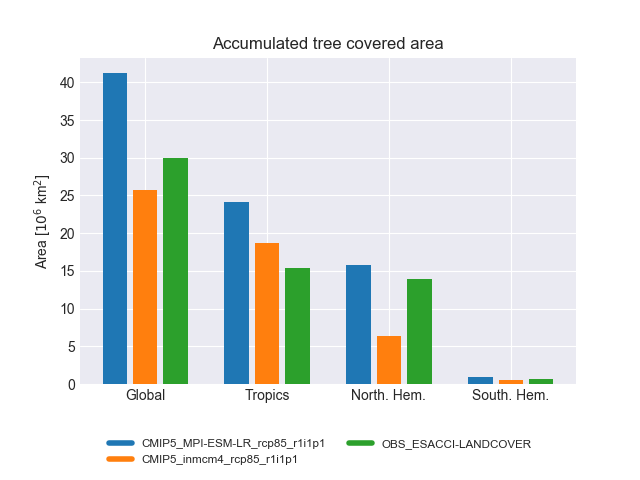
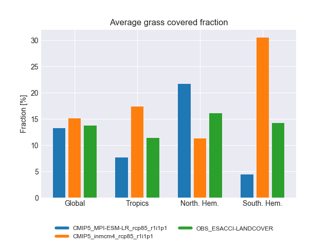
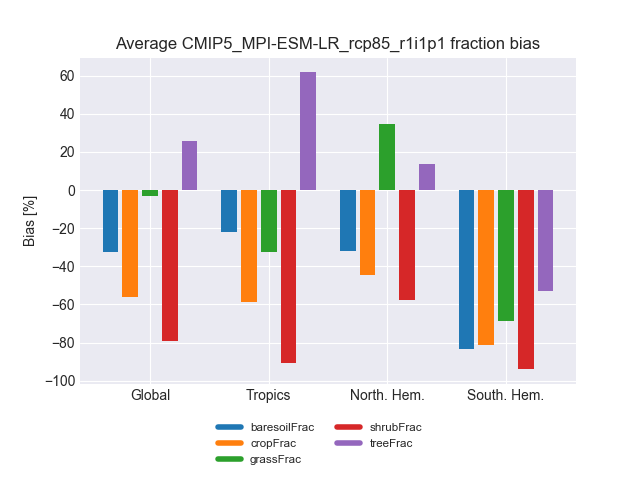
The diagnostic computes the accumulated and fractional extent of major land cover classes, namely bare soil, crops, grasses, shrubs and trees. The numbers are compiled for the whole land surface as well as separated into Tropics, northern Extratropics and southern Extratropics. The cover fractions are compared to ESA-CCI land cover data.
Available recipes and diagnostics
Recipes are stored in recipes/
recipe_landcover.yml
Diagnostics are stored in diag_scripts/landcover/
landcover.py: bar plots showing the accumulated area and mean fractional coverage for five land cover classes for all experiments as well as their bias compared to observations.
User settings
script landcover.py
Required settings for script
reference_dataset: land cover extent dataset for comparison. The script was developed using ESACCI-LANDCOVER observations.
Optional settings for script
comparison: [variable, model] Choose whether one plot per land cover class is generated comparing the different experiments (default) or one plot per model comparing the different land cover classes.
colorscheme: Plotstyle used for the bar plots. A list of available style is found at https://matplotlib.org/gallery/style_sheets/style_sheets_reference.html. Seaborn is used as default.
Variables
baresoilFrac (land, monthly mean, time latitude longitude)
grassFrac (land, monthly mean, time latitude longitude)
treeFrac (land, monthly mean, time latitude longitude)
shrubFrac (land, monthly mean, time latitude longitude)
cropFrac (land, monthly mean, time latitude longitude)
Observations and reformat scripts
ESA-CCI land cover data (Defourny et al., 2015) needs to be downloaded manually by the user and converted to netCDF files containing the grid cell fractions for the five major land cover types. The data and a conversion tool are available at https://maps.elie.ucl.ac.be/CCI/viewer/ upon registration. After obtaining the data and the user tool, the remapping to 0.5 degree can be done with:
./bin/aggregate-map.sh
-PgridName=GEOGRAPHIC_LAT_LON
-PnumRows=360
-PoutputLCCSClasses=true
-PnumMajorityClasses=0
ESACCI-LC-L4-LCCS-Map-300m-P1Y-2015-v2.0.7b.nc
Next, the data needs to be aggregated into the five major classes (PFT) similar to the study of Georgievski & Hagemann (2018) and converted from grid cell fraction into percentage.
PFT |
ESA-CCI Landcover Classes |
|---|---|
baresoilFrac |
Bare_Soil |
cropFrac |
Managed_Grass |
grassFrac |
Natural_Grass |
shrubFrac |
Shrub_Broadleaf_Deciduous + Shrub_Broadleaf_Evergreen + Shrub_Needleleaf_Evergreen |
treeFrac |
Tree_Broadleaf_Deciduous + Tree_Broadleaf_Evergreen + Tree_Needleleaf_Deciduous + Tree_Needleleaf_Evergreen |
Finally, it might be necessary to adapt the grid structure to the experiments files, e.g converting the -180 –> 180 degree grid to 0 –> 360 degree and inverting the order of latitudes. Note, that all experiments will be regridded onto the grid of the land cover observations, thus it is recommended to convert to the coarses resolution which is sufficient for the planned study. For the script development, ESA-CCI data on 0.5 degree resolution was used with land cover data averaged over the 2008-2012 period.
References
Defourny et al. (2015): ESA Land Cover Climate Change Initiative (ESA LC_cci) data: ESACCI-LC-L4-LCCS-Map-300m-P5Y-[2000,2005,2010]-v1.6.1 via Centre for Environmental Data Analysis
Georgievski, G. & Hagemann, S. Characterizing uncertainties in the ESA-CCI land cover map of the epoch 2010 and their impacts on MPI-ESM climate simulations, Theor Appl Climatol (2018). https://doi.org/10.1007/s00704-018-2675-2