Emergent constraints for equilibrium climate sensitivity
Overview
Calculates equilibrium climate sensitivity (ECS) versus
S index, D index and lower tropospheric mixing index (LTMI); similar to fig. 5 from Sherwood et al. (2014)
southern ITCZ index and tropical mid-tropospheric humidity asymmetry index; similar to fig. 2 and 4 from Tian (2015)
covariance of shortwave cloud reflection (Brient and Schneider, 2016)
climatological Hadley cell extent (Lipat et al., 2017)
temperature variability metric; similar to fig. 2 from Cox et al. (2018)
total cloud fraction difference between tropics and mid-latitudes; similar to fig. 3 from Volodin (2008)
response of marine boundary layer cloud (MBLC) fraction changes to sea surface temperature (SST); similar to fig. 3 of Zhai et al. (2015)
Cloud shallowness index (Brient et al., 2016)
Error in vertically-resolved tropospheric zonal average relative humidity (Su et al., 2014)
The results are displayed as scatterplots.
Note
The recipe recipe_ecs_scatter.yml requires pre-calulation of the
equilibrium climate sensitivites (ECS) for all models. The ECS values are
calculated with recipe_ecs.yml. The netcdf file containing the ECS values
(path and filename) is specified by diag_script_info@ecs_file.
Alternatively, the netcdf file containing the ECS values can be generated
with the cdl-script
$diag_scripts/emergent_constraints/ecs_cmip.cdl (recommended method):
save script given at the end of this recipe as ecs_cmip.cdl
run command: ncgen -o ecs_cmip.nc ecs_cmip.cdl
copy ecs_cmip.nc to directory given by diag_script_info@ecs_file (e.g. $diag_scripts/emergent_constraints/ecs_cmip.nc)
Available recipes and diagnostics
Recipes are stored in recipes/
recipe_ecs_scatter.yml
recipe_ecs_constraints.yml
Diagnostics are stored in diag_scripts
emergent_constraints/ecs_scatter.ncl: calculate emergent constraints for ECS
emergent_constraints/ecs_scatter.py: calculate further emergent constraints for ECS
emergent_constraints/univariate_constraint.py: create scatterplots for emergent constraints
climate_metrics/psi.py: calculate temperature variabililty metric (Cox et al., 2018)
User settings in recipe
Script emergent_constraints/ecs_scatter.ncl
Required settings (scripts)
diag: emergent constraint to calculate (“itczidx”, “humidx”, “ltmi”, “covrefl”, “shhc”, “sherwood_d”, “sherwood_s”)
ecs_file: path and filename of netCDF containing precalculated ECS values (see note above)
Optional settings (scripts)
calcmm: calculate multi-model mean (True, False)
legend_outside: plot legend outside of scatterplots (True, False)
output_diag_only: Only write netcdf files for X axis (True) or write all plots (False)
output_models_only: Only write models (no reference datasets) to netcdf files (True, False)
output_attributes: Additonal attributes for all output netcdf files
predef_minmax: use predefined internal min/max values for axes (True, False)
styleset: “CMIP5” (if not set, diagnostic will create a color table and symbols for plotting)
suffix: string to add to output filenames (e.g.”cmip3”)
Required settings (variables)
reference_dataset: name of reference data set
Optional settings (variables)
none
Color tables
none
Script emergent_constraints/ecs_scatter.py
Required settings (scripts)
diag: emergent constraint to calculate (“brient_shal”, “su”, “volodin”, “zhai”)
Optional settings (scripts)
metric: Metric to measure model error, only relevant for Su et al. (2014) constraint (“regression_slope”, “correlation_coefficient”)
output_attributes: Additonal attributes for all output netcdf files
pattern: Only accept ancestor files that match that pattern
savefig_kwargs: Keyword arguments for matplotlib.pyplot’s
savefig()function, see https://matplotlib.org/3.2.0/api/_as_gen/matplotlib.pyplot.savefig.htmlseaborn_settings: Options for seaborn’s
set()methods (affects all plots), see https://seaborn.pydata.org/generated/seaborn.set.html
Required settings (variables)
reference_dataset: name of reference data set
Optional settings (variables)
none
Script emergent_constraints/univariate_constraint.py
All input data for this diagnostic must be marked with a
var_type(eitherfeature,label,prediction_inputorprediction_input_error) and atag, which describes the data. This diagnostic supports only a singletagforlabelandfeature. For everytag, areference_datasetcan be specified, which will be automatically considered asprediction_input. Ifreference_datasetcontains'|'(e.g.'OBS1|OBS2'), mutliple datasets are considered asprediction_input(in this case'OBS1'and'OBS2').Required settings (scripts)
none
Optional settings (scripts)
all_data_label: Label used in plots when all input data is considered. Only relevant if
group_byis not usedconfidence_level: Confidence level for estimation of constrained target variable.
group_by: Group input data by an attribute (e.g. produces separate plots for the individual groups, etc.)
ignore_patterns: Ignore ancestor files that match that patterns
merge_identical_pred_input: Use identical prediction_input values as single value
numbers_as_markers: Use numbers as markers in scatterplots
patterns: Only accept ancestor files that match that patterns
read_external_file: Read input datasets from external file given as absolute path or relative path. In the latter case,
'auxiliary_data_dir'from the user configuration file is used as base directorysavefig_kwargs: Keyword arguments for matplotlib.pyplot’s
savefig()function, see https://matplotlib.org/3.2.0/api/_as_gen/matplotlib.pyplot.savefig.htmlseaborn_settings: Options for seaborn’s
set()methods (affects all plots), see https://seaborn.pydata.org/generated/seaborn.set.html
Required settings (variables)
reference_dataset: name of reference data set
Optional settings (variables)
none
Script climate_metrics/psi.py
See Emergent constraint on equilibrium climate sensitivity from global temperature variability.
Variables
cl (atmos, monthly mean, longitude latitude level time)
clt (atmos, monthly mean, longitude latitude time)
pr (atmos, monthly mean, longitude latitude time)
hur (atmos, monthly mean, longitude latitude level time)
hus (atmos, monthly mean, longitude latitude level time)
rsdt (atmos, monthly mean, longitude latitude time)
rsut (atmos, monthly mean, longitude latitude time)
rsutcs (atmos, monthly mean, longitude latitude time)
rtnt or rtmt (atmos, monthly mean, longitude latitude time)
ta (atmos, monthly mean, longitude latitude level time)
tas (atmos, monthly mean, longitude latitude time)
tasa (atmos, monthly mean, longitude latitude time)
tos (atmos, monthly mean, longitude latitude time)
ts (atmos, monthly mean, longitude latitude time)
va (atmos, monthly mean, longitude latitude level time)
wap (atmos, monthly mean, longitude latitude level time)
zg (atmos, monthly mean, longitude latitude time)
Observations and reformat scripts
Note
Obs4mips data can be used directly without any preprocessing.
See headers of reformat scripts for non-obs4mips data for download instructions.
AIRS (obs4mips): hus, husStderr
AIRS-2-0 (obs4mips): hur
CERES-EBAF (obs4mips): rsdt, rsut, rsutcs
ERA-Interim (OBS6): hur, ta, va, wap
GPCP-SG (obs4mips): pr
HadCRUT4 (OBS): tasa
HadISST (OBS): ts
MLS-AURA (OBS6): hur
TRMM-L3 (obs4mips): pr, prStderr
References
Brient, F., and T. Schneider, J. Climate, 29, 5821-5835, doi:10.1175/JCLIM-D-15-0897.1, 2016.
Brient et al., Clim. Dyn., 47, doi:10.1007/s00382-015-2846-0, 2016.
Cox et al., Nature, 553, doi:10.1038/nature25450, 2018.
Gregory et al., Geophys. Res. Lett., 31, doi:10.1029/2003GL018747, 2004.
Lipat et al., Geophys. Res. Lett., 44, 5739-5748, doi:10.1002/2017GL73151, 2017.
Sherwood et al., nature, 505, 37-42, doi:10.1038/nature12829, 2014.
Su, et al., J. Geophys. Res. Atmos., 119, doi:10.1002/2014JD021642, 2014.
Tian, Geophys. Res. Lett., 42, 4133-4141, doi:10.1002/2015GL064119, 2015.
Volodin, Izvestiya, Atmospheric and Oceanic Physics, 44, 288-299, doi:10.1134/S0001433808030043, 2008.
Zhai, et al., Geophys. Res. Lett., 42, doi:10.1002/2015GL065911, 2015.
Example plots
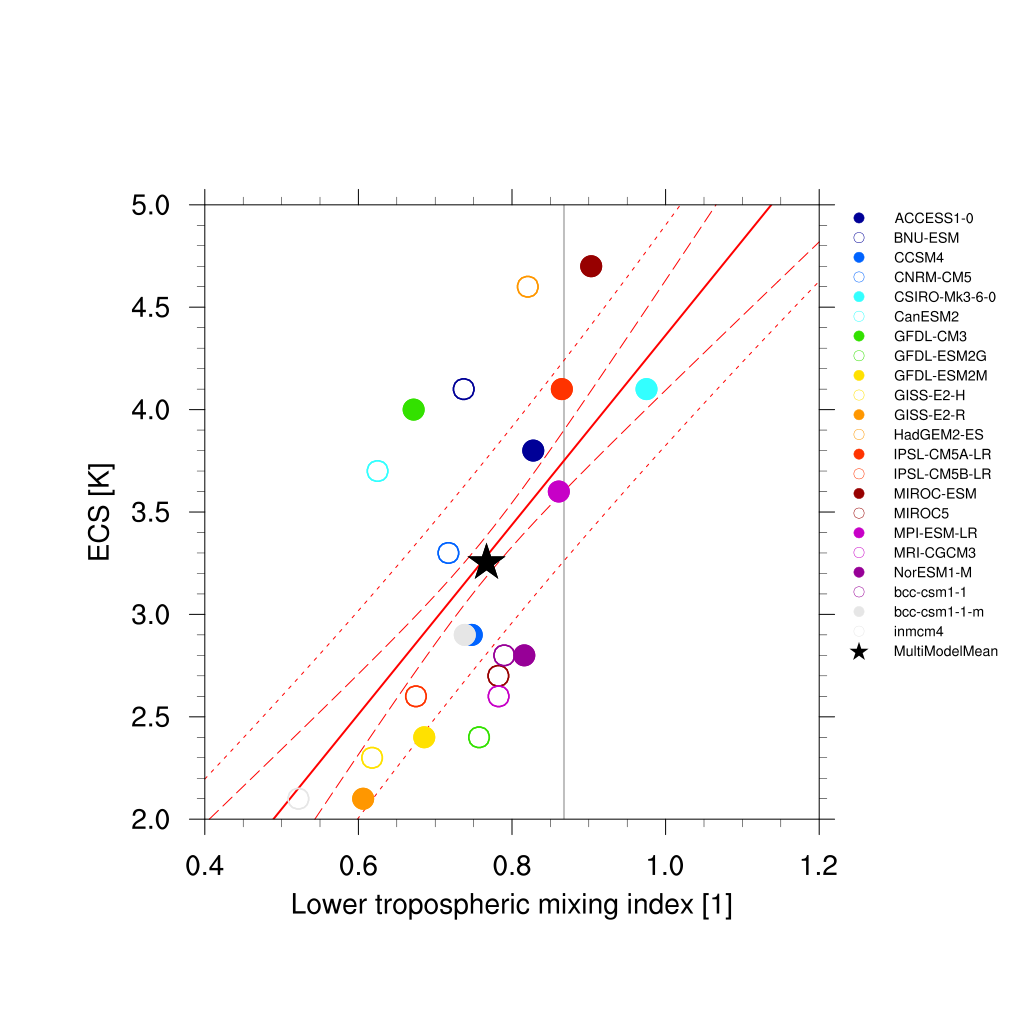
Fig. 64 Lower tropospheric mixing index (LTMI; Sherwood et al., 2014) vs. equilibrium climate sensitivity from CMIP5 models.
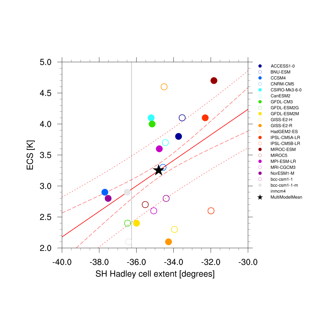
Fig. 65 Climatological Hadley cell extent (Lipat et al., 2017) vs. equilibrium climate sensitivity from CMIP5 models.
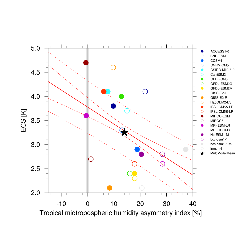
Fig. 66 Tropical mid-tropospheric humidity asymmetry index (Tian, 2015) vs. equilibrium climate sensitivity from CMIP5 models.
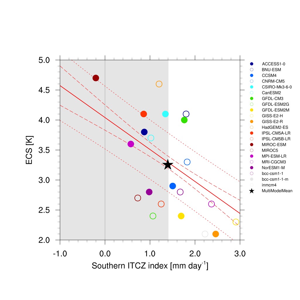
Fig. 67 Southern ITCZ index (Tian, 2015) vs. equilibrium climate sensitivity from CMIP5 models.
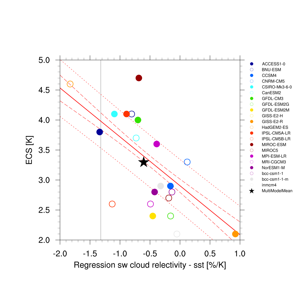
Fig. 68 Covariance of shortwave cloud reflection (Brient and Schneider, 2016) vs. equilibrium climate sensitivity from CMIP5 models.

Fig. 69 Difference in total cloud fraction between tropics (28°S - 28°N) and Southern midlatitudes (56°S - 36°S) (Volodin, 2008) vs. equilibrium climate sensitivity from CMIP5 models.