Emergent constraint on equilibrium climate sensitivity from global temperature variability
Overview
This recipe reproduces the emergent constraint proposed by Cox et al. (2018) for the equilibrium climate sensitivity (ECS) using global temperature variability. The latter is defined by a metric which can be calculated from the global temperature variance (in time) \(\sigma_T\) and the one-year-lag autocorrelation of the global temperature \(\alpha_{1T}\) by
Using the simple Hasselmann model they show that this quantity is linearly correlated with the ECS. Since it only depends on the temporal evolution of the global surface temperature, there is lots of observational data available which allows the construction of an emergent relationship. This method predicts an ECS range of 2.2K to 3.4K (66% confidence limit).
Available recipes and diagnostics
Recipes are stored in recipes/
recipe_cox18nature.yml
Diagnostics are stored in diag_scripts/
emergent_constraints/cox18nature.py
climate_metrics/ecs.py
climate_metrics/psi.py
User settings in recipe
Preprocessor
area_statistics(operation: mean): Calculate global mean.
Script emergent_constraints/cox18nature.py
confidence_level, float, optional (default: 0.66): Confidence level for ECS error estimation.
Script climate_metrics/ecs.py
read_external_file, str, optional: Read ECS and net climate feedback parameter from external file. All other input data is ignored.
Script climate_metrics/psi.py
output_attributes, dict, optional: Write additional attributes to all output netcdf files.lag, int, optional (default: 1): Lag (in years) for the autocorrelation function.window_length, int, optional (default: 55): Number of years used for the moving window average.
Variables
tas (atmos, monthly, longitude, latitude, time)
tasa (atmos, monthly, longitude, latitude, time)
References
Cox, Peter M., Chris Huntingford, and Mark S. Williamson. “Emergent constraint on equilibrium climate sensitivity from global temperature variability.” Nature 553.7688 (2018): 319.
Example plots
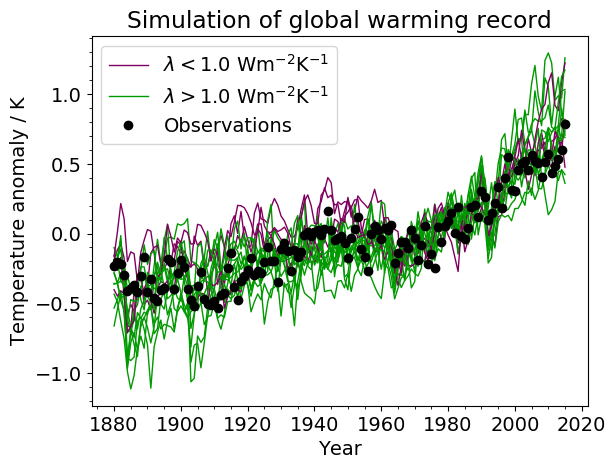
Fig. 74 Simulated change in global temperature from CMIP5 models (coloured lines), compared to the global temperature anomaly from the HadCRUT4 dataset (black dots). The anomalies are relative to a baseline period of 1961–1990. The model lines are colour-coded, with lower-sensitivity models (λ > 1 Wm-2K-1) shown by green lines and higher-sensitivity models (λ < 1 Wm-2K-1) shown by magenta lines.
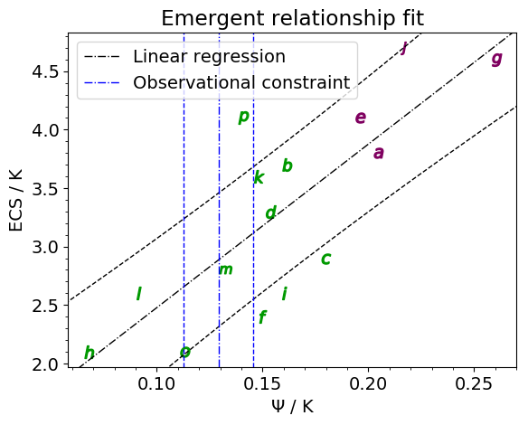
Fig. 75 Emergent relationship between ECS and the ψ metric. The black dot-dashed line shows the best-fit linear regression across the model ensemble, with the prediction error for the fit given by the black dashed lines. The vertical blue lines show the observational constraint from the HadCRUT4 observations: the mean (dot-dashed line) and the mean plus and minus one standard deviation (dashed lines).
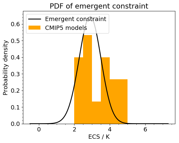
Fig. 76 The PDF for ECS. The orange histograms (both panels) show the prior distributions that arise from equal weighting of the CMIP5 models in 0.5 K bins.