Recipe for evaluating Arctic Ocean
Overview
The Arctic ocean is one of the areas of the Earth where the effects of climate change are especially visible today. Two most prominent processes are Arctic amplification [e.g. Serreze and Barry, 2011] and decrease of the sea ice area and thickness. Both receive good coverage in the literature and are already well-studied. Much less attention is paid to the interior of the Arctic Ocean itself. In order to increase our confidence in projections of the Arctic climate future proper representation of the Arctic Ocean hydrography is necessary.
The main focus of this diagnostics is evaluation of ocean components of climate models in the Arctic Ocean, however most of the diagnostics are implemented in a way that can be easily expanded to other parts of the World Ocean. Most of the diagnostics aim at model comparison to climatological data (PHC3), so we target historical CMIP simulations. However scenario runs also can be analysed to have an impression of how Arcti Ocean hydrography will chnage in the future.
At present only the subset of CMIP models can be used in particular because our analysis is limited to z coordinate models.
Available recipes
Recipe is stored in recipes/
recipe_arctic_ocean.yml : contains all setting nessesary to run diagnostics and metrics.
Currenly the workflow do not allow to easily separate diagnostics from each other, since some of the diagnostics rely on the results of other diagnostics. The recipe currently do not use preprocessor options, so input files are CMORised monthly mean 3D ocean varibales on original grid.
The following plots will be produced by the recipe:
Hovmoeller diagrams
The characteristics of vertical TS distribution can change with time, and consequently the vertical TS distribution is an important indicator of the behaviour of the coupled ocean-sea ice-atmosphere system in the North Atlantic and Arctic Oceans. One way to evaluate these changes is by using Hovmoller diagrams. Hovmoller diagrams for two main Arctic Ocean basins – Eurasian and Amerasian with T and S spatially averaged on a monthly basis for every vertical level are available. This diagnostic allows the temporal evolution of vertical ocean potential temperature distribution to be assessed.
Related settings in the recipe:
# Define regions, as a list.
# 'EB' - Eurasian Basin of the Arctic Ocean
# 'AB' - Amerasian Basin of the Arctic Ocean
# 'Barents_sea' - Barrents Sea
# 'North_sea'   - North Sea
hofm_regions: ["AB" ,  'EB']
# Define variables to use, should also be in "variables"
# entry of your diagnostic
hofm_vars: ['thetao', 'so']
# Maximum depth of Hovmoeller and vertical profiles
hofm_depth: 1500
# Define if Hovmoeller diagrams will be ploted.
hofm_plot: True
# Define colormap (as a list, same size as list with variables)
# Only cmaps from matplotlib and cmocean are supported.
# Additional cmap - 'custom_salinity1'.
hofm_cmap: ['Spectral_r', 'custom_salinity1']
# Data limits for plots,
# List of the same size as the list of the variables
# each entry is [vmin, vmax, number of levels, rounding limit]
hofm_limits: [[-2, 2.3, 41, 1], [30.5, 35.1, 47, 2]]
# Number of columns in the plot
hofm_ncol: 3
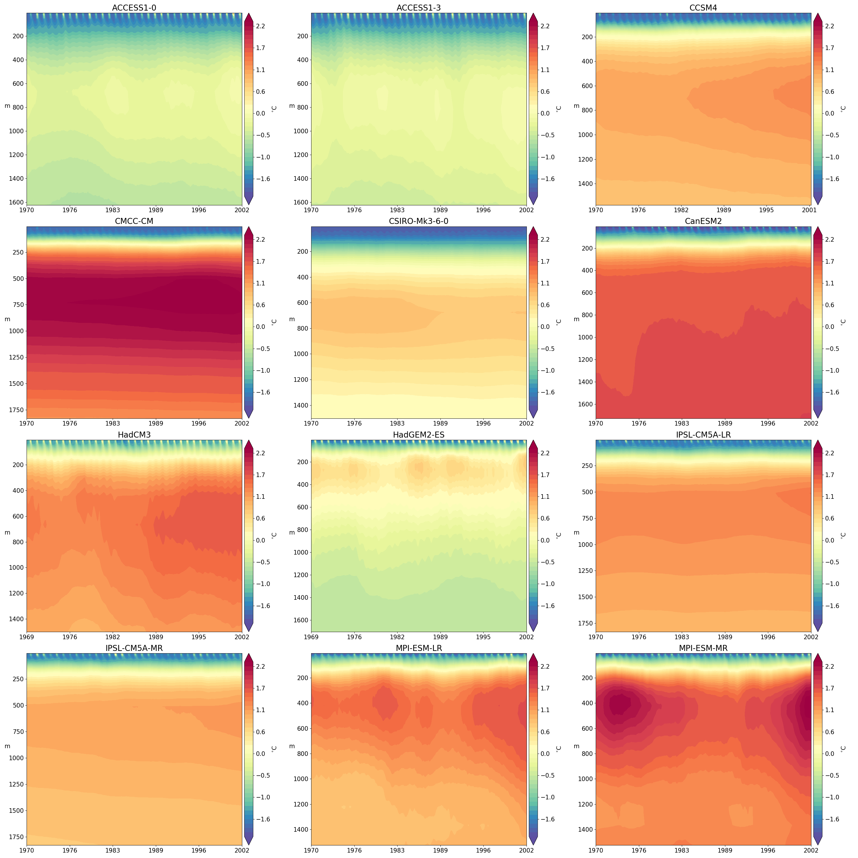
Fig. 128 Hovmoller diagram of monthly spatially averaged potential temperature in the Eurasian Basin of the Arctic Ocean for selected CMIP5 climate models (1970-2005).
Vertical profiles
The vertical structure of temperature and salinity (T and S) in the ocean model is a key diagnostic that is used for ocean model evaluation. Realistic T and S distributions means that model properly represent dynamic and thermodynamic processes in the ocean. Different ocean basins have different hydrological regimes so it is important to perform analysis of vertical TS distribution for different basins separately. The basic diagnostic in this sense is mean vertical profiles of temperature and salinity over some basin averaged for relatively long period of time. In addition to individual vertical profiles for every model, we also show the mean over all participating models and similar profile from climatological data (PHC3).
Several settings for vertical profiles (region, variables, maximum depths) will be determined by the Hovmoeller diagram settings. The reason is that vertical profiles are calculated from Hovmoeller diagram data. Mean vertical profile is calculated by lineraly interpolating data on standard WOA/PHC depths.
Related settings in the recipe:
# Define regions, as a list.
# 'EB' - Eurasian Basin of the Arctic Ocean
# 'AB' - Amerasian Basin of the Arctic Ocean
# 'Barents_sea' - Barrents Sea
# 'North_sea'   - North Sea
hofm_regions: ["AB" ,  'EB']
# Define variables to use, should also be in "variables" entry of your diagnostic
hofm_vars: ['thetao', 'so']
# Maximum depth of Hovmoeller and vertical profiles
hofm_depth: 1500
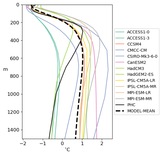
Fig. 129 Mean (1970-2005) vertical potential temperature distribution in the Eurasian basin for participating CMIP5 coupled ocean models, PHC3 climatology (dotted red line) and multi-model mean (dotted black line).
Spatial distribution maps of variables
The spatial distribution of basic oceanographic variables characterises the properties and spreading of ocean water masses. For the coupled models, capturing the spatial distribution of oceanographic variables is especially important in order to correctly represent the ocean-ice-atmosphere interface. We have implemented plots with spatial maps of temperature and salinity at original model levels.
Plots spatial distribution of variables at selected depths in North Polar projection on original model grid. For plotting the model depths that are closest to provided plot2d_depths will be selected. Settings allow to define color maps and limits for each variable individually. Color maps should be ehter part of standard matplotlib set or one of the cmocean color maps. Additional colormap custom_salinity1 is provided.
Related settings in the recipe:
# Depths for spatial distribution maps
plot2d_depths: [10, 100]
# Variables to plot spatial distribution maps
plot2d_vars: ['thetao', 'so']
# Define colormap (as a list, same size as list with variables)
# Only cmaps from matplotlib and cmocean are supported.
# Additional cmap - 'custom_salinity1'.
plot2d_cmap: ['Spectral_r', 'custom_salinity1']
# Data limits for plots,
# List of the same size as the list of the variables
# each entry is [vmin, vmax, number of levels, rounding limit]
plot2d_limits: [[-2, 4, 20, 1], [30.5, 35.1, 47, 2]]
# number of columns for plots
plot2d_ncol: 3
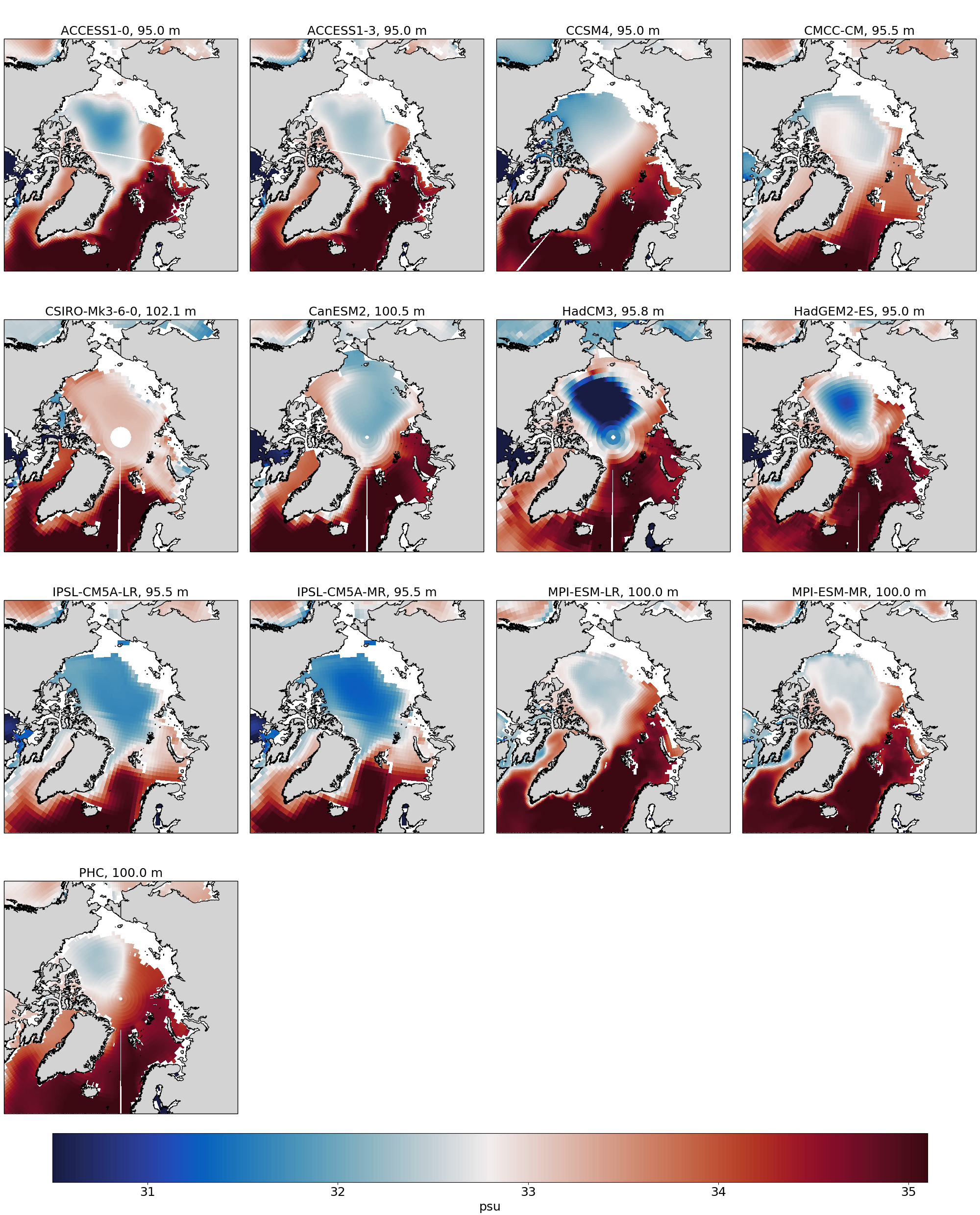
Fig. 130 Mean (1970-2005) salinity distribution at 100 meters.
Spatial distribution maps of biases
For temperature and salinity, we have implemented spatial maps of model biases from the observed climatology. For the model biases, values from the original model levels are linearly interpolated to the climatology and then spatially interpolated from the model grid to the regular PHC (climatology) grid. Resulting fields show model performance in simulating spatial distribution of temperature and salinity.
Related settings in the recipe:
plot2d_bias_depths: [10, 100]
# Variables to plot spatial distribution of the bias for.
plot2d_bias_vars: ['thetao', 'so']
# Color map names for every variable
plot2d_bias_cmap: ['balance', 'balance']
# Data limits for plots,
# List of the same size as the list of the variables
# each entry is [vmin, vmax, number of levels, rounding limit]
plot2d_bias_limits: [[-3, 3, 20, 1], [-2, 2, 47, 2]]
# number of columns in the bias plots
plot2d_bias_ncol: 3
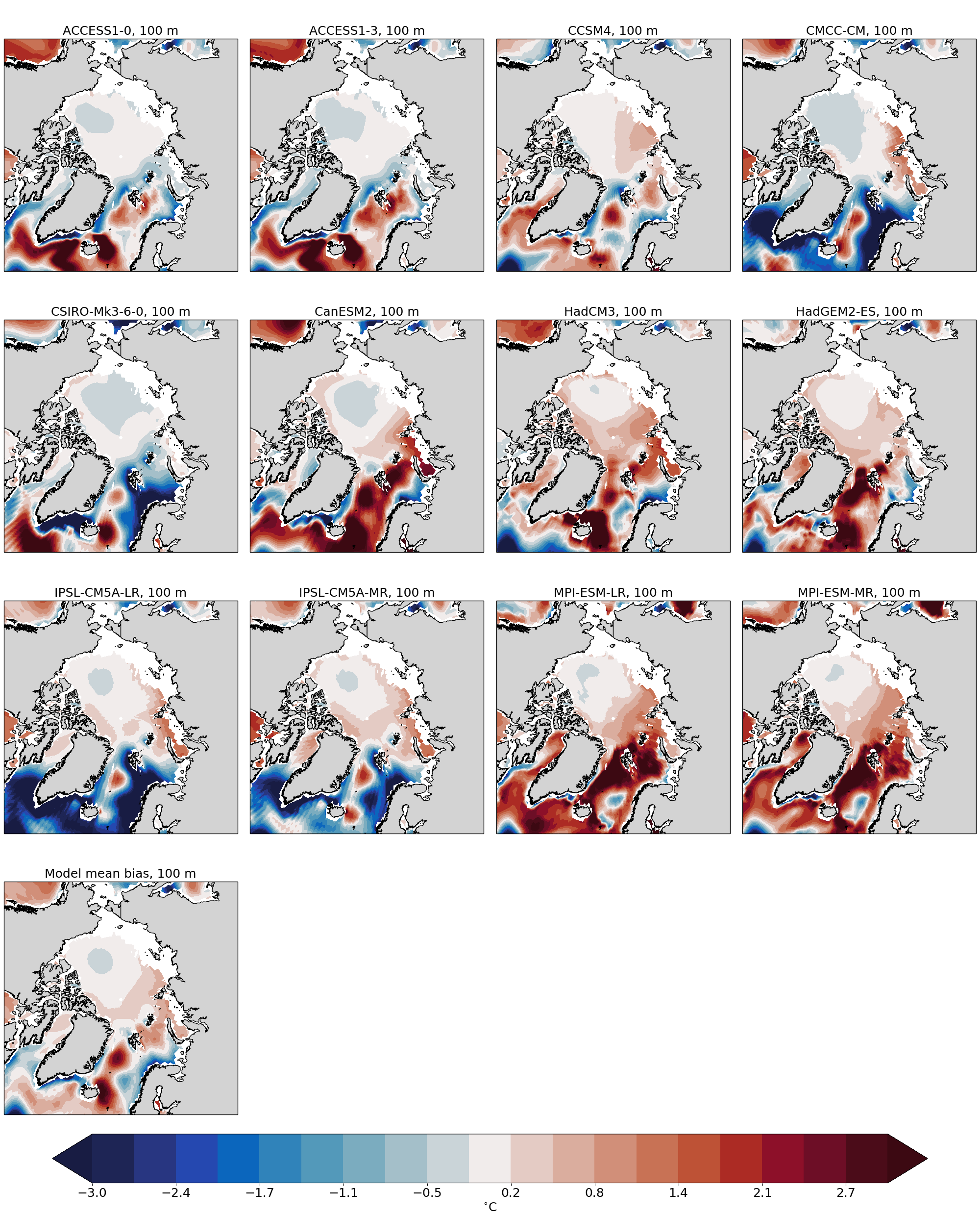
Fig. 131 Mean (1970-2005) salinity bias at 100m relative to PHC3 climatology
Transects
Vertical transects through arbitrary sections are important for analysis of vertical distribution of ocean water properties and especially useful when exchange between different ocean basins is evaluated. We have implemented diagnostics that allow for the definition of an arbitrary ocean section by providing set of points on the ocean surface. For each point, a vertical profile on the original model levels is interpolated. All profiles are then connected to form a transect. The great-circle distance between the points is calculated and used as along-track distance.
One of the main use cases is to create vertical sections across ocean passages, for example Fram Strait.
Plots transect maps for pre-defined set of transects (defined in regions.py, see below). The transect_depth defines maximum depth of the transect. Transects are calculated from data averaged over the whole time period.
Related settings in the recipe:
# Select regions (transects) to plot
# Available options are:
# AWpath - transect along the path of the Atlantic Water
# Fram - Fram strait
transects_regions: ["AWpath", "Fram"]
# Variables to plot on transects
transects_vars: ['thetao', 'so']
# Color maps for every variable
transects_cmap: ['Spectral_r', 'custom_salinity1']
# Data limits for plots,
# List of the same size as the list of the variables
# each entry is [vmin, vmax, number of levels, rounding limit]
transects_limits: [[-2, 4, 20, 1], [30.5, 35.1, 47, 2]]
# Maximum depth to plot the data
transects_depth: 1500
# number of columns
transects_ncol: 3
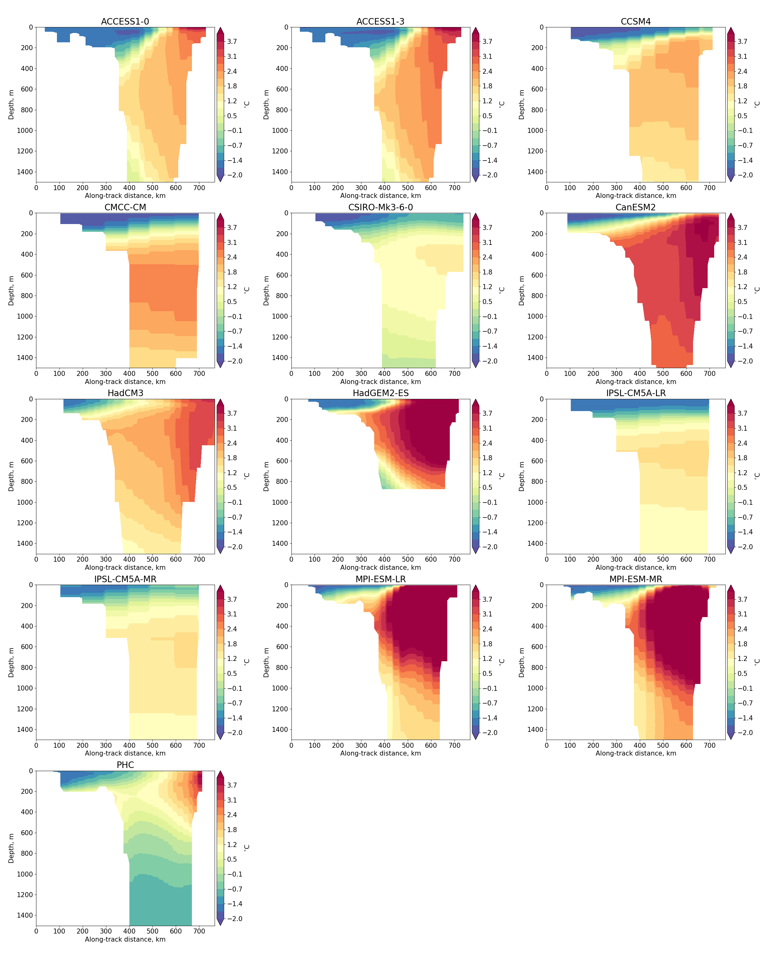
Fig. 132 Mean (1970-2005) potential temperature across the Fram strait.
Atlantic Water core depth and temperature
Atlantic water is a key water mass of the Arctic Ocean and its proper representation is one of the main challenges in Arctic Ocean modelling. We have created two metrics by which models can be easily compared in terms of Atlantic water simulation. The temperature of the Atlantic Water core is calculated for every model as the maximum potential temperature between 200 and 1000 meters depth in the Eurasian Basin. The depth of the Atlantic Water core is calculated as the model level depth where the maximum temperature is found in Eurasian Basin (Atlantic water core temperature).
The AW core depth and temperature will be calculated from data generated for Hovmoeller diagrams for EB region, so it should be selected in the Hovmoeller diagrams settings as one of the hofm_regions.
In order to evaluate the spatial distribution of Atlantic water in different climate models we also provide diagnostics with maps of the spatial temperature distribution at model’s Atlantic Water depth.
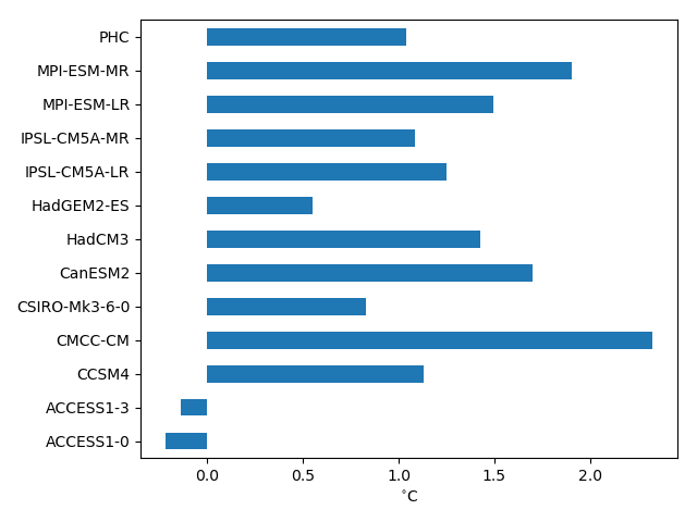
Fig. 133 Mean (1970-2005) Atlantic Water core temperature. PHC33 is an observed climatology.
TS-diagrams
T-S diagrams combine temperature and salinity, which allows the analysis of water masses and their potential for mixing. The lines of constant density for specific ranges of temperature and salinity are shown on the background of the T-S diagram. The dots on the diagram are individual grid points from specified region at all model levels within user specified depth range.
Related settings in the recipe:
tsdiag_regions: ["AB" ,  'EB']
# Maximum depth to consider data for TS diagrams
tsdiag_depth: 1500
# Number of columns
tsdiag_ncol: 3
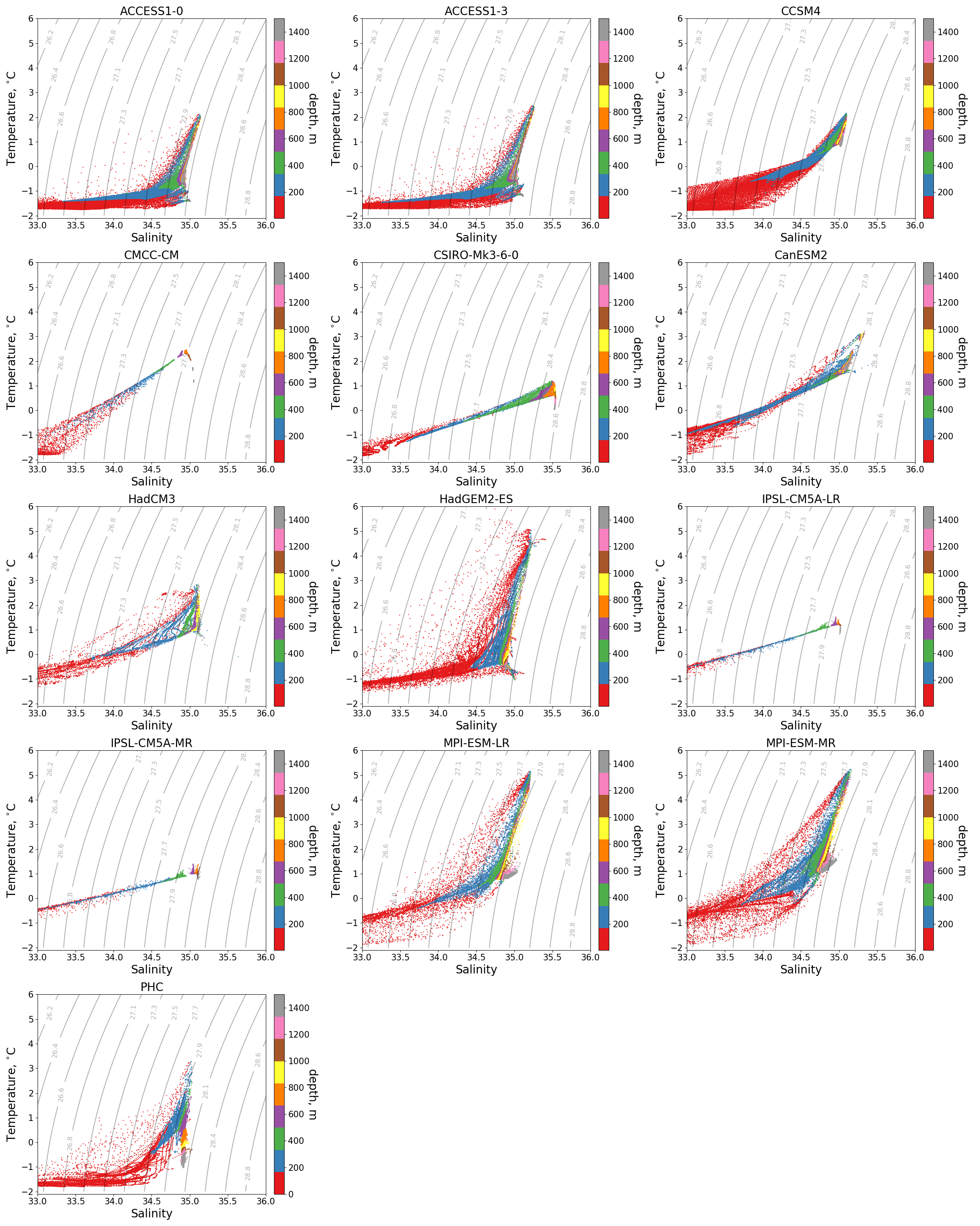
Fig. 134 Mean (1970-2005) T-S diagrams for Eurasian Basin of the Arctic Ocean.
Available diagnostics
The following python modules are included in the diagnostics package:
arctic_ocean.py : Reads settings from the recipe and call functions to do analysis and plots.
getdata.py : Deals with data preparation.
interpolation.py : Include horizontal and vertical interpolation functions specific for ocean models.
plotting.py : Ocean specific plotting functions
regions.py : Contains code to select specific regions, and definition of the regions themselves.
utils.py : Helpful utilites.
Diagnostics are stored in diag_scripts/arctic_ocean/
Variables
thetao (ocean, monthly, longitude, latitude, time)
so (ocean, monthly, longitude, latitude, time)
Observations and reformat scripts
PHC3 climatology
References
Ilıcak, M. et al., An assessment of the Arctic Ocean in a suite of interannual CORE-II simulations. Part III: Hydrography and fluxes, Ocean Modelling, Volume 100, April 2016, Pages 141-161, ISSN 1463-5003, doi.org/10.1016/j.ocemod.2016.02.004
Steele, M., Morley, R., & Ermold, W. (2001). PHC: A global ocean hydrography with a high-quality Arctic Ocean. Journal of Climate, 14(9), 2079-2087.
Wang, Q., et al., An assessment of the Arctic Ocean in a suite of interannual CORE-II simulations. Part I: Sea ice and solid freshwater, Ocean Modelling, Volume 99, March 2016, Pages 110-132, ISSN 1463-5003, doi.org/10.1016/j.ocemod.2015.12.008
Wang, Q., Ilicak, M., Gerdes, R., Drange, H., Aksenov, Y., Bailey, D. A., … & Cassou, C. (2016). An assessment of the Arctic Ocean in a suite of interannual CORE-II simulations. Part II: Liquid freshwater. Ocean Modelling, 99, 86-109, doi.org/10.1016/j.ocemod.2015.12.009