Loading, processing, and visualizing data

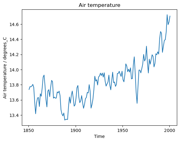
This notebook shows how to load a dataset, use the preprocessor functions, and visualize the result. In this notebook we will plot the annual mean temperature from 1850 till 2100 from one model.

%matplotlib inline

import matplotlib.pyplot as plt
import iris.quickplot

from esmvalcore.config import CFG
from esmvalcore.dataset import Dataset
from esmvalcore.esgf import download, ESGFFile
from esmvalcore.preprocessor import area_statistics, annual_statistics

Configure ESMValCore so it searches the ESGF for data

CFG['search_esgf'] = 'when_missing'

Define the dataset we are going to use. In this case surface air temperature (tas).

tas = Dataset(
    short_name='tas',
    mip='Amon',
    project='CMIP5',
    dataset='MPI-ESM-MR',
    ensemble='r1i1p1',
    exp='historical',
    timerange='1850/2000',
)
tas

Dataset:
{'dataset': 'MPI-ESM-MR',
 'project': 'CMIP5',
 'mip': 'Amon',
 'short_name': 'tas',
 'ensemble': 'r1i1p1',
 'exp': 'historical',
 'timerange': '1850/2000'}

In order to compute the area average later on, we add the cell areas (areacella) as a supplementary dataset. This will append a new dataset to the list of supplementary datasets. Its facets are copied from the tas dataset and updated with the provided facets:

tas.add_supplementary(short_name='areacella', mip='fx', ensemble='r0i0p0')
tas.supplementaries

[Dataset:
 {'dataset': 'MPI-ESM-MR',
  'project': 'CMIP5',
  'mip': 'fx',
  'short_name': 'areacella',
  'ensemble': 'r0i0p0',
  'exp': 'historical',
  'timerange': '1850/2000'}]

ESMValCore can automatically add extra facets based on the project, mip, short_name, and dataset. These extra facets are automatically added and used when searching for input files.

tas.augment_facets()
tas

Dataset:
{'dataset': 'MPI-ESM-MR',
 'project': 'CMIP5',
 'mip': 'Amon',
 'short_name': 'tas',
 'ensemble': 'r1i1p1',
 'exp': 'historical',
 'frequency': 'mon',
 'institute': ['MPI-M'],
 'long_name': 'Near-Surface Air Temperature',
 'modeling_realm': ['atmos'],
 'original_short_name': 'tas',
 'product': ['output1', 'output2'],
 'standard_name': 'air_temperature',
 'timerange': '1850/2000',
 'units': 'K'}
supplementaries:
  {'dataset': 'MPI-ESM-MR',
   'project': 'CMIP5',
   'mip': 'fx',
   'short_name': 'areacella',
   'ensemble': 'r0i0p0',
   'exp': 'historical',
   'frequency': 'fx',
   'institute': ['MPI-M'],
   'long_name': 'Atmosphere Grid-Cell Area',
   'modeling_realm': ['atmos', 'land'],
   'original_short_name': 'areacella',
   'product': ['output1', 'output2'],
   'standard_name': 'cell_area',
   'units': 'm2'}
session: 'session-686367c0-001c-4864-839d-c20887cf7415_20230301_160531'

Use the find_files method to find the files corresponding to the dataset.

tas.find_files()
print(tas.files)
for supplementary_ds in tas.supplementaries:
    print(supplementary_ds.files)

[ESGFFile:cmip5/output1/MPI-M/MPI-ESM-MR/historical/mon/atmos/Amon/r1i1p1/v20120503/tas_Amon_MPI-ESM-MR_historical_r1i1p1_185001-200512.nc on hosts ['aims3.llnl.gov', 'esgf.ceda.ac.uk', 'esgf.nci.org.au', 'esgf1.dkrz.de']]
[ESGFFile:cmip5/output1/MPI-M/MPI-ESM-MR/historical/fx/atmos/fx/r0i0p0/v20120503/areacella_fx_MPI-ESM-MR_historical_r0i0p0.nc on hosts ['aims3.llnl.gov', 'esgf.ceda.ac.uk', 'esgf.nci.org.au', 'esgf1.dkrz.de']]

If the files are not available locally, ESMValCore can download them for us.

files = list(tas.files)
for supplementary_ds in tas.supplementaries:
    files.extend(supplementary_ds.files)
files = [file for file in files if isinstance(file, ESGFFile)]
download(files, CFG['download_dir'])
tas.find_files()
print(tas.files)
for supplementary_ds in tas.supplementaries:
    print(supplementary_ds.files)

[LocalFile('~/climate_data/cmip5/output1/MPI-M/MPI-ESM-MR/historical/mon/atmos/Amon/r1i1p1/v20120503/tas_Amon_MPI-ESM-MR_historical_r1i1p1_185001-200512.nc')]
[LocalFile('~/climate_data/cmip5/output1/MPI-M/MPI-ESM-MR/historical/fx/atmos/fx/r0i0p0/v20120503/areacella_fx_MPI-ESM-MR_historical_r0i0p0.nc')]

The data in the files can be loaded into an iris.cube.Cube. ESMValCore will automatically check for and fix problems with the data formatting and attach the cell area.

cube = tas.load()
cube

Air Temperature (K)	time	latitude	longitude
Shape	1812	96	192
Dimension coordinates
time	x	-	-
latitude	-	x	-
longitude	-	-	x
Cell measures
cell_area	-	x	x
Scalar coordinates
height	2.0 m
Cell methods
mean	time
Attributes
Conventions	'CF-1.4'
associated_files	'baseURL: http://cmip-pcmdi.llnl.gov/CMIP5/dataLocation gridspecFile: gridspec_atmos_fx_MPI-ESM-MR_historical_r0i0p0.nc ...'
branch_time	0.0
cmor_version	'2.6.0'
contact	'cmip5-mpi-esm@dkrz.de'
experiment	'historical'
experiment_id	'historical'
forcing	'GHG,Oz,SD,Sl,Vl,LU'
frequency	'mon'
initialization_method	1
institute_id	'MPI-M'
institution	'Max Planck Institute for Meteorology'
model_id	'MPI-ESM-MR'
modeling_realm	'atmos'
parent_experiment	'N/A'
parent_experiment_id	'N/A'
parent_experiment_rip	'N/A'
physics_version	1
product	'output'
project_id	'CMIP5'
realization	1
references	'ECHAM6: n/a; JSBACH: Raddatz et al., 2007. Will the tropical land biosphere ...'
source	'MPI-ESM-MR 2011; URL: http://svn.zmaw.de/svn/cosmos/branches/releases/mpi-esm-cmip5/src/mod; ...'
table_id	'Table Amon (27 April 2011) a5a1c518f52ae340313ba0aada03f862'
title	'MPI-ESM-MR model output prepared for CMIP5 historical'

cell_area = cube.cell_measures()[0]
cell_area

<CellMeasure: cell_area / (m2)  <lazy>  shape(96, 192)>

This code shows how to use some esmvalcore.preprocessor functions to compute the global annual mean temperature in degrees Celsius:

cube = area_statistics(cube, operator='mean')
cube = annual_statistics(cube, operator='mean')
cube.convert_units('degrees_C')

The iris.quickplot module has useful functions for quickly plotting the results:

iris.quickplot.plot(cube)
plt.show()