IPCC AR6 Chapter 3 (selected figures)
Overview
This recipe collects selected diagnostics used in IPCC AR6 WGI Chapter 3: Human influence on the climate system. Plots from IPCC AR6 can be readily reproduced and compared to previous versions. The aim is to be able to start with what was available now the next time allowing us to focus on developing more innovative analysis methods rather than constantly having to “re-invent the wheel”.
The plots are produced collecting the diagnostics from individual recipes. The following figures from Eyring et al. (2021) can currently be reproduced:
Figure 3.3 a,b,c,d: Surface Air Temperature - Model Bias
Figure 3.4: Anomaly Of Near-Surface Air Temperature
Figure 3.5: Temporal Variability Of Near-Surface Air Temperature
Figure 3.13: Precipitation - Model Bias
Figure 3.15: Precipitation Anomaly
Available recipes and diagnostics
Recipes are stored in esmvaltool/recipes/ipccwg1ar6ch3/
recipe_ipccwg1ar6ch3_atmosphere.yml
Diagnostics are stored in esmvaltool/diag_scripts/
Fig. 3.3:
ipcc_ar5/ch12_calc_IAV_for_stippandhatch.ncl: See here:.
ipcc_ar6/model_bias.ncl
Fig. 3.4:
ipcc_ar6/tas_anom.ncl
ipcc_ar6/tsline_collect.ncl
Fig. 3.5:
ipcc_ar6/zonal_st_dev.ncl
Fig. 3.13:
ipcc_ar5/ch12_calc_IAV_for_stippandhatch.ncl: See here:.
ipcc_ar6/model_bias.ncl
Fig. 3.15:
ipcc_ar6/precip_anom.ncl
User settings in recipe
Script ipcc_ar5/ch12_calc_IAV_for_stippandhatch.ncl
See here.
Script ipcc_ar6/model_bias.ncl
Optional settings (scripts)
plot_abs_diff: additionally also plot absolute differences (true, false)
plot_rel_diff: additionally also plot relative differences (true, false)
plot_rms_diff: additionally also plot root mean square differences (true, false)
projection: map projection, e.g., Mollweide, Mercator
timemean: time averaging, i.e. “seasonalclim” (DJF, MAM, JJA, SON), “annualclim” (annual mean)
Required settings (variables)
reference_dataset: name of reference dataset
Color tables
variable “tas” and “tos”: diag_scripts/shared/plot/rgb/ipcc-ar6_temperature_div.rgb, diag_scripts/shared/plot/rgb/ipcc-ar6_temperature_10.rgb, diag_scripts/shared/plot/rgb/ipcc-ar6_temperature_seq.rgb
variable “pr”: diag_scripts/shared/plots/rgb/ipcc-ar6_precipitation_seq.rgb, diag_scripts/shared/plot/rgb/ipcc-ar6_precipitation_10.rgb
variable “sos”: diag_scripts/shared/plot/rgb/ipcc-ar6_misc_seq_1.rgb, diag_scripts/shared/plot/rgb/ipcc-ar6_misc_div.rgb
Script ipcc_ar6/tas_anom.ncl
Required settings for script
styleset: as in diag_scripts/shared/plot/style.ncl functions
Optional settings for script
blending: if true, calculates blended surface temperature
ref_start: start year of reference period for anomalies
ref_end: end year of reference period for anomalies
ref_value: if true, right panel with mean values is attached
ref_mask: if true, model fields will be masked by reference fields
region: name of domain
plot_units: variable unit for plotting
y-min: set min of y-axis
y-max: set max of y-axis
header: if true, region name as header
volcanoes: if true, adds volcanoes to the plot
write_stat: if true, write multi model statistics in nc-file
Optional settings for variables
reference_dataset: reference dataset; REQUIRED when calculating anomalies
Color tables
e.g. diag_scripts/shared/plot/styles/cmip5.style
Script ipcc_ar6/tsline_collect.ncl
Optional settings for script
blending: if true, then var=”gmst” otherwise “gsat”
ref_start: start year of reference period for anomalies
ref_end: end year of reference period for anomalies
region: name of domain
plot_units: variable unit for plotting
y-min: set min of y-axis
y-max: set max of y-axis
order: order in which experiments should be plotted
stat_shading: if true: shading of statistic range
ref_shading: if true: shading of reference period
Optional settings for variables
reference_dataset: reference dataset; REQUIRED when calculating anomalies
Script ipcc_ar6/zonal_st_dev.ncl
Required settings for script
styleset: as in diag_scripts/shared/plot/style.ncl functions
Optional settings for script
plot_legend: if true, plot legend will be plotted
plot_units: variable unit for plotting
multi_model_mean: if true, multi-model mean and uncertaintiy will be plotted
Optional settings for variables
reference_dataset: reference dataset; REQUIRED when calculating anomalies
Script ipcc_ar6/precip_anom.ncl
Required settings for script
panels: list of variables plotted in each panel
start_year: start of time coordinate
end_year: end of time coordinate
Optional settings for script
anomaly: true if anomaly should be calculated
ref_start: start year of reference period for anomalies
ref_end: end year of reference period for anomalies
ref_mask: if true, model fields will be masked by reference fields
region: name of domain
plot_units: variable unit for plotting
header: if true, region name as header
stat: statistics for multi model nc-file (MinMax,5-95,10-90)
y_min: set min of y-axis
y_max: set max of y-axis
Variables
pr (atmos, monthly mean, longitude latitude time)
tas (atmos, monthly mean, longitude latitude time)
tasa (atmos, monthly mean, longitude latitude time)
Observations and reformat scripts
BerkeleyEarth (tasa - esmvaltool/cmorizers/data/formatters/datasets/berkeleyearth.py)
CRU (pr - esmvaltool/cmorizers/data/formatters/datasets/cru.py)
ERA5 (tas - ERA5 data can be used via the native6 project)
GHCN (pr - esmvaltool/cmorizers/data/formatters/datasets/ghcn.ncl)
GPCP-SG (pr - obs4MIPs)
HadCRUT5 (tasa - esmvaltool/cmorizers/data/formatters/datasets/hadcrut5.py)
Kadow2020 (tasa - esmvaltool/cmorizers/data/formatters/datasets/kadow2020.py)
NOAAGlobalTemp (tasa - esmvaltool/cmorizers/data/formatters/datasets/noaaglobaltemp.py)
References
Eyring, V., N.P. Gillett, K.M. Achuta Rao, R. Barimalala, M. Barreiro Parrillo, N. Bellouin, C. Cassou, P.J. Durack, Y. Kosaka, S. McGregor, S. Min, O. Morgenstern, and Y. Sun, 2021: Human Influence on the Climate System. In Climate Change 2021: The Physical Science Basis. Contribution of Working Group I to the Sixth Assessment Report of the Intergovernmental Panel on Climate Change [Masson-Delmotte, V., P. Zhai, A. Pirani, S.L. Connors, C. Péan, S. Berger, N. Caud, Y. Chen, L. Goldfarb, M.I. Gomis, M. Huang, K. Leitzell, E. Lonnoy, J.B.R. Matthews, T.K. Maycock, T. Waterfield, O. Yelekçi, R. Yu, and B. Zhou (eds.)]. Cambridge University Press. In Press.
Example plots
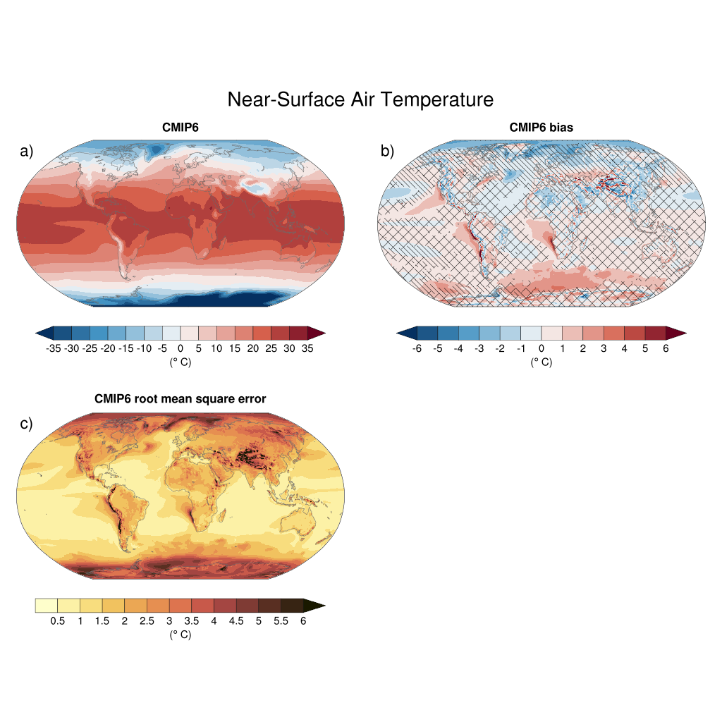
Fig. 121 Figure 3.3: Annual mean near-surface (2 m) air temperature (°C) for the period 1995–2014. (a) Multi-model (ensemble) mean constructed with one realization of the CMIP6 historical experiment from each model. (b) Multi-model mean bias, defined as the difference between the CMIP6 multi-model mean and the climatology of the fifth generation European Centre for Medium-Range Weather Forecasts (ECMWF) atmospheric reanalysis of the global climate (ERA5). (c) Multi-model mean of the root mean square error calculated over all months separately and averaged, with respect to the climatology from ERA5. Uncertainty is represented using the advanced approach: No overlay indicates regions with robust signal, where ≥66% of models show change greater than the variability threshold and ≥80% of all models agree on sign of change; diagonal lines indicate regions with no change or no robust signal, where <66% of models show a change greater than the variability threshold; crossed lines indicate regions with conflicting signal, where ≥66% of models show change greater than the variability threshold and <80% of all models agree on sign of change.
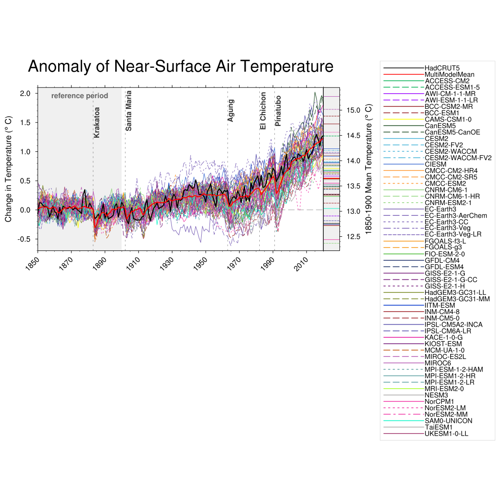
Fig. 122 Figure 3.4a: Observed and simulated time series of the anomalies in annual and global mean surface air temperature (GSAT). All anomalies are differences from the 1850–1900 time-mean of each individual time series. The reference period 1850–1900 is indicated by grey shading. (a) Single simulations from CMIP6 models (thin lines) and the multi-model mean (thick red line). Observational data (thick black lines) are from the Met Office Hadley Centre/Climatic Research Unit dataset (HadCRUT5), and are blended surface temperature (2 m air temperature over land and sea surface temperature over the ocean). All models have been subsampled using the HadCRUT5 observational data mask. Vertical lines indicate large historical volcanic eruptions. Inset: GSAT for each model over the reference period, not masked to any observations.
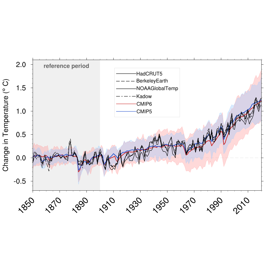
Fig. 123 Figure 3.4b: Observed and simulated time series of the anomalies in annual and global mean surface air temperature (GSAT). All anomalies are differences from the 1850–1900 time-mean of each individual time series. The reference period 1850–1900 is indicated by grey shading. (b) Multi-model means of CMIP5 (blue line) and CMIP6 (red line) ensembles and associated 5th to 95th percentile ranges (shaded regions). Observational data are HadCRUT5, Berkeley Earth, National Oceanic and Atmospheric Administration NOAAGlobalTemp and Kadow et al. (2020). Masking was done as in (a). CMIP6 historical simulations were extended with SSP2-4.5 simulations for the period 2015–2020 and CMIP5 simulations were extended with RCP4.5 simulations for the period 2006–2020. All available ensemble members were used. The multi-model means and percentiles were calculated solely from simulations available for the whole time span (1850–2020).
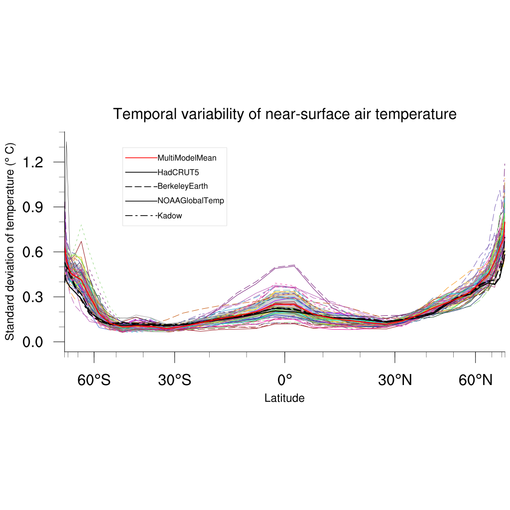
Fig. 124 Figure 3.5: The standard deviation of annually averaged zonal-mean near-surface air temperature. This is shown for four detrended observed temperature datasets (HadCRUT5, Berkeley Earth, NOAAGlobalTemp and Kadow et al. (2020), for the years 1995-2014) and 59 CMIP6 pre-industrial control simulations (one ensemble member per model, 65 years) (after Jones et al., 2013). For line colours see the legend of Figure 3.4. Additionally, the multi-model mean (red) and standard deviation (grey shading) are shown. Observational and model datasets were detrended by removing the least-squares quadratic trend.
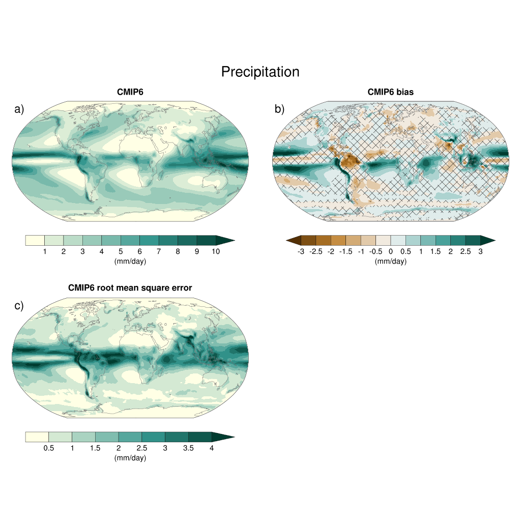
Fig. 125 Figure 3.13: Annual-mean precipitation rate (mm day–1) for the period 1995–2014. (a) Multi-model (ensemble) mean constructed with one realization of the CMIP6 historical experiment from each model. (b) Multi-model mean bias, defined as the difference between the CMIP6 multi-model mean and precipitation analysis from the Global Precipitation Climatology Project (GPCP) version 2.3 (Adler et al., 2003). (c) Multi-model mean of the root mean square error calculated over all months separately and averaged with respect to the precipitation analysis from GPCP version 2.3. Uncertainty is represented using the advanced approach. No overlay indicates regions with robust signal, where ≥66% of models show change greater than the variability threshold and ≥80% of all models agree on sign of change; diagonal lines indicate regions with no change or no robust signal, where <66% of models show a change greater than the variability threshold; crossed lines indicate regions with conflicting signal, where ≥66% of models show change greater than the variability threshold and <80% of all models agree on the sign of change.
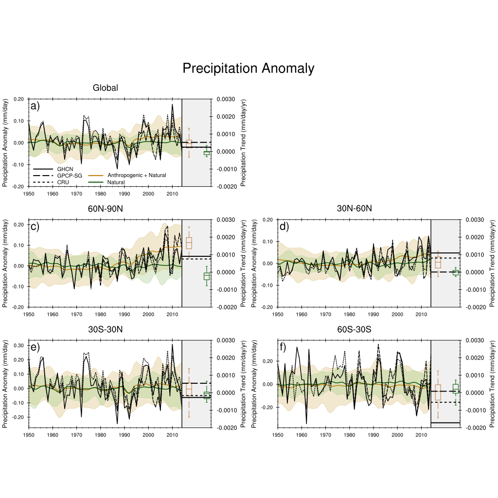
Fig. 126 Figure 3.15: Observed and simulated time series of anomalies in zonal average annual mean precipitation. (a), (c–f) Evolution of global and zonal average annual mean precipitation (mm day–1) over areas of land where there are observations, expressed relative to the base period of 1961–1990, simulated by CMIP6 models (one ensemble member per model) forced with both anthropogenic and natural forcings (brown) and natural forcings only (green). Multi-model means are shown in thick solid lines and shading shows the 5–95% confidence interval of the individual model simulations. The data is smoothed using a low pass filter. Observations from three different datasets are included: gridded values derived from Global Historical Climatology Network (GHCN version 2) station data, updated from Zhang et al. (2007), data from the Global Precipitation Climatology Product (GPCP L3 version 2.3, Adler et al. (2003)) and from the Climate Research Unit (CRU TS4.02, Harris et al. (2014)). Also plotted are boxplots showing interquartile and 5–95% ranges of simulated trends over the period for simulations forced with both anthropogenic and natural forcings (brown) and natural forcings only (blue). Observed trends for each observational product are shown as horizontal lines. Panel (b) shows annual mean precipitation rate (mm day–1) of GHCN version 2 for the years 1950–2014 over land areas used to compute the plots.