ClimWIP: independence & performance weighting

Overview

This recipe calculates weights based on combined performance and independence metrics. These weights can be used in subsequent diagnostics. Reference implementation based on https://github.com/lukasbrunner/ClimWIP

Available recipes and diagnostics

Recipes are stored in esmvaltool/recipes/

• recipe_climwip_test_basic.yml

• recipe_climwip_test_performance_sigma.yml

(A recipe adding a ‘real’ case will be added in due time.)

Diagnostics are stored in esmvaltool/diag_scripts/weighting/climwip/

• main.py: Compute weights for each input dataset

• calibrate_sigmas.py: Compute the sigma values on the fly

• core_functions.py: A collection of core functions used by the scripts

• io_functions.py: A collection of input/output functions used by the scripts

Plot scripts are stored in esmvaltool/diag_scripts/weighting/

• weighted_temperature_graph.py: Show the difference between weighted and non-weighted temperature anomalies as time series.

• weighted_temperature_map.py: Show the difference between weighted and non-weighted temperature anomalies as map.

• plot_utilities.py: A collection of functions use by the plot scripts.

User settings in recipe

1. Script main.py

Required settings for script

• performance_sigma xor calibrate_performance_sigma: If performance_contributions is given exactly one of the two has to be given. Otherwise they can be skipped or not set.

  • performance_sigma: float setting the shape parameter for the performance weights calculation (determined offline).

  • calibrate_performance_sigma: dictionary setting the performance sigma calibration. Has to contain at least the key-value pair specifying target: variable_group. Optional parameters for adjusting the calibration are not yet implemented. WARNING: It is highly recommended to visually inspect the graphical output of the calibration to check if everything worked as intended. In case the calibration fails, the best performance sigma will still be indicated in the figure (see example Fig. 8 below) but not automatically picked - the user can decide to use it anyway by setting it in the recipe (not recommenced).

• independence_sigma: float setting the shape parameter for the independence weights calculation (determined offline). Can be skipped or not set if independence_contributions is skipped or not set.

• performance_contributions: dictionary where the keys represent the variable groups to be included in the performance calculation. The values give the relative contribution of each group, with 0 being equivalent to not including the group. Can be skipped or not set then weights will be based purely on model independence (this is mutually exclusive with independence_contributions being skipped or not set).

• independence_contributions: dictionary where the keys represent the variable groups to be included in the independence calculation. The values give the relative contribution of each group, with 0 being equivalent to not including the group. Can be skipped or not set then weights will be based purely on model performance (this is mutually exclusive with performance_contributions being skipped or not set).

• combine_ensemble_members: set to true if ensemble members of the same model should be combined during the processing (leads to identical weights for all ensemble members of the same model). Recommended if running with many (>10) ensemble members per model.

• obs_data: list of project names to specify which are the the observational data. The rest is assumed to be model data.

Required settings for variables

• This script takes multiple variables as input as long as they’re available for all models

• start_year: provide the period for which to compute performance and independence.

• end_year: provide the period for which to compute performance and independence.

• mip: typically Amon

• preprocessor: e.g. climwip_summer_mean

• additional_datasets: provide a list of model data for performance calculation.

Required settings for preprocessor

• Different combinations of preprocessor functions can be used, but the end result should always be aggregated over the time dimension, i.e. the input for the diagnostic script should be 2d (lat/lon).

Optional settings for preprocessor

• extract_region or extract_shape can be used to crop the input data.

• extract_season can be used to focus on a single season.

• different climate statistics can be used to calculate mean or (detrended) std_dev.

2. Script weighted_temperature_graph.py

Required settings for script

• ancestors: must include weights from previous diagnostic

• weights: the filename of the weights: ‘weights.nc’

Required settings for variables

• This script only takes temperature (tas) as input

• start_year: provide the period for which to plot a temperature change graph.

• end_year: provide the period for which to plot a temperature change graph.

• mip: typically Amon

• preprocessor: temperature_anomalies

Required settings for preprocessor

• Different combinations of preprocessor functions can be used, but the end result should always be aggregated over the latitude and longitude dimensions, i.e. the input for the diagnostic script should be 1d (time).

Optional settings for preprocessor

• Can be a global mean or focus on a point, region or shape

• Anomalies can be calculated with respect to a custom reference period

• Monthly, annual or seasonal average/extraction can be used

3. Script weighted_temperature_map.py

   Required settings for script

   • ancestors: must include weights from previous diagnostic

   • weights: the filename of the weights: ‘weights_combined.nc’

   Optional settings for script

   • model_aggregation: how to aggregate the models: mean (default), median, integer between 0 and 100 given a percentile

   • xticks: positions to draw xticks at

   • yticks: positions to draw yticks at

   Required settings for variables

   • This script takes temperature (tas) as input

   • start_year: provide the period for which to plot a temperature change graph.

   • end_year: provide the period for which to plot a temperature change graph.

   • mip: typically Amon

   • preprocessor: temperature_anomalies

   Optional settings for variables

   • A second variable is optional: temperature reference (tas_reference). If given, maps of temperature change to the reference are drawn, otherwise absolute temperature are drawn.

   • tas_reference takes the same fields as tas

Variables

• pr (atmos, monthly mean, longitude latitude time)

• tas (atmos, monthly mean, longitude latitude time)

• psl (atmos, monthly mean, longitude latitude time)

• more variables can be added if available for all datasets.

Observations and reformat scripts

Observation data is defined in a separate section in the recipe and may include multiple datasets.

References

• Brunner et al. 2020, Earth Syst. Dynam., 11, 995-1012,.

• Merrifield et al. 2020, Earth Syst. Dynam., 11, 807-834,.

• Brunner et al. 2019, Environ. Res. Lett., 14, 124010,.

• Lorenz et al. 2018, J. Geophys. Res.: Atmos., 9, 4509-4526,.

• Knutti et al. 2017, Geophys. Res. Lett., 44, 1909-1918,.

Example plots

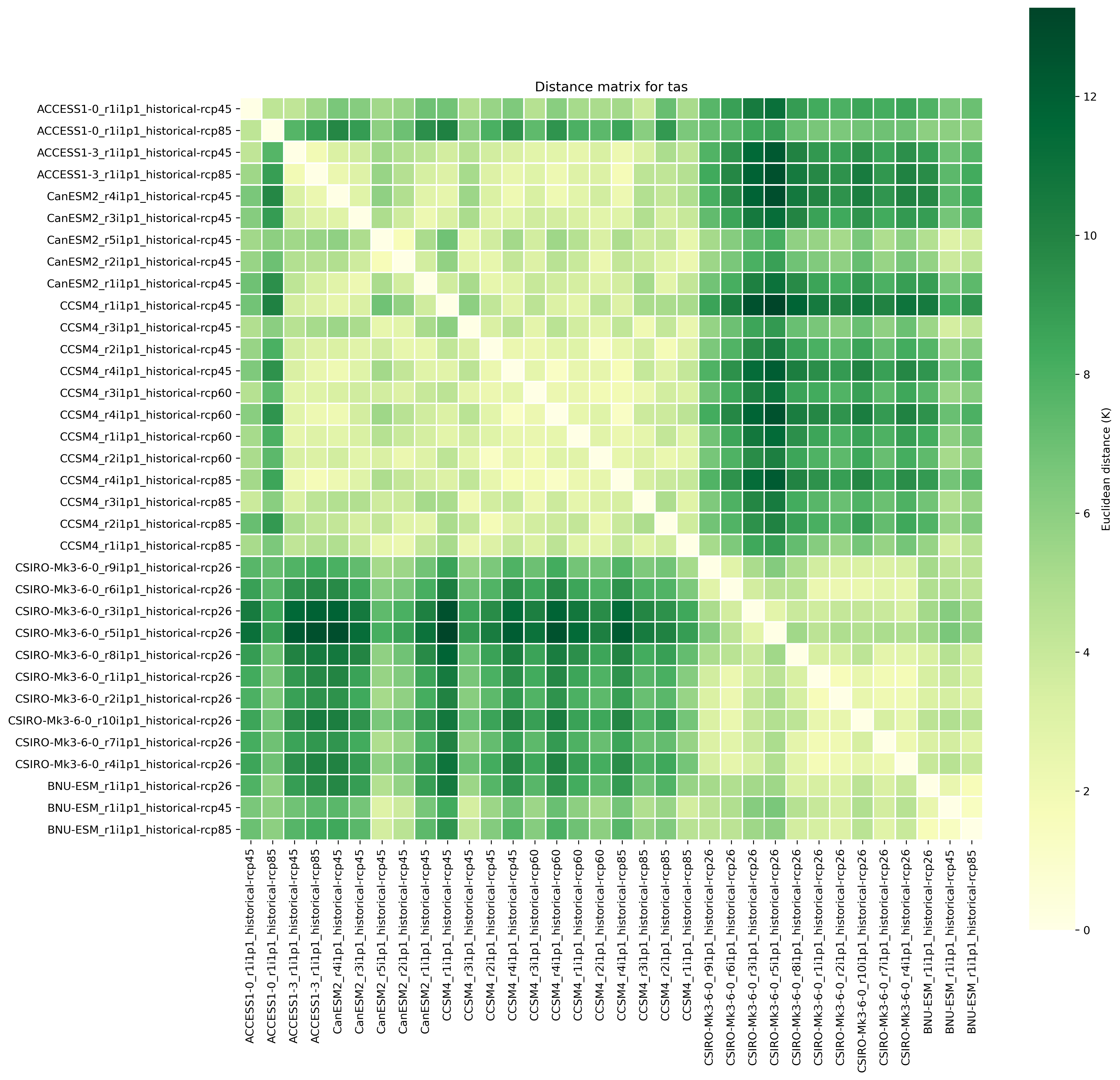
Fig. 4 Distance matrix for temperature, providing the independence metric.

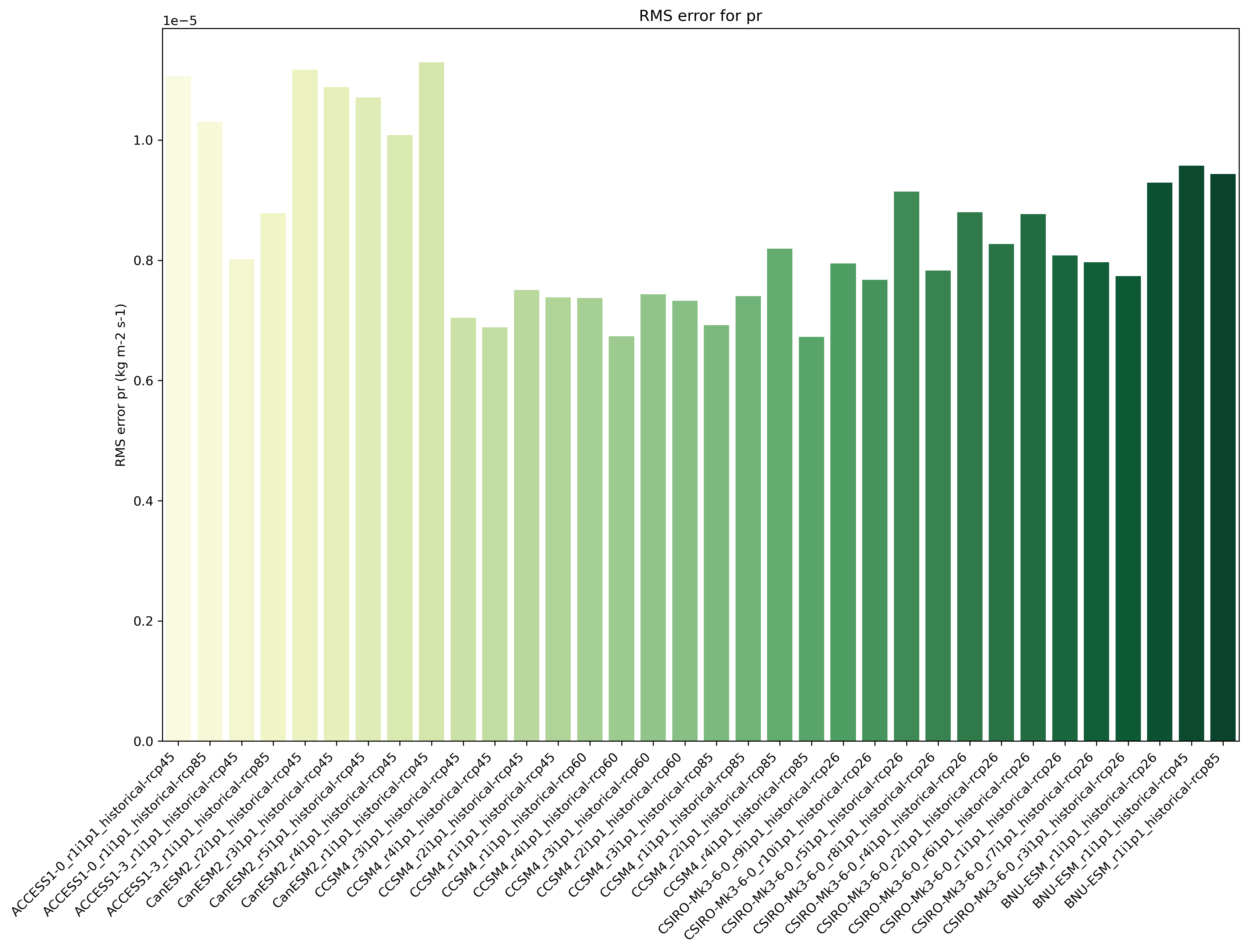
Fig. 5 Distance of preciptation relative to observations, providing the performance metric.

Fig. 6 Weights determined by combining independence and performance metrics for tas.

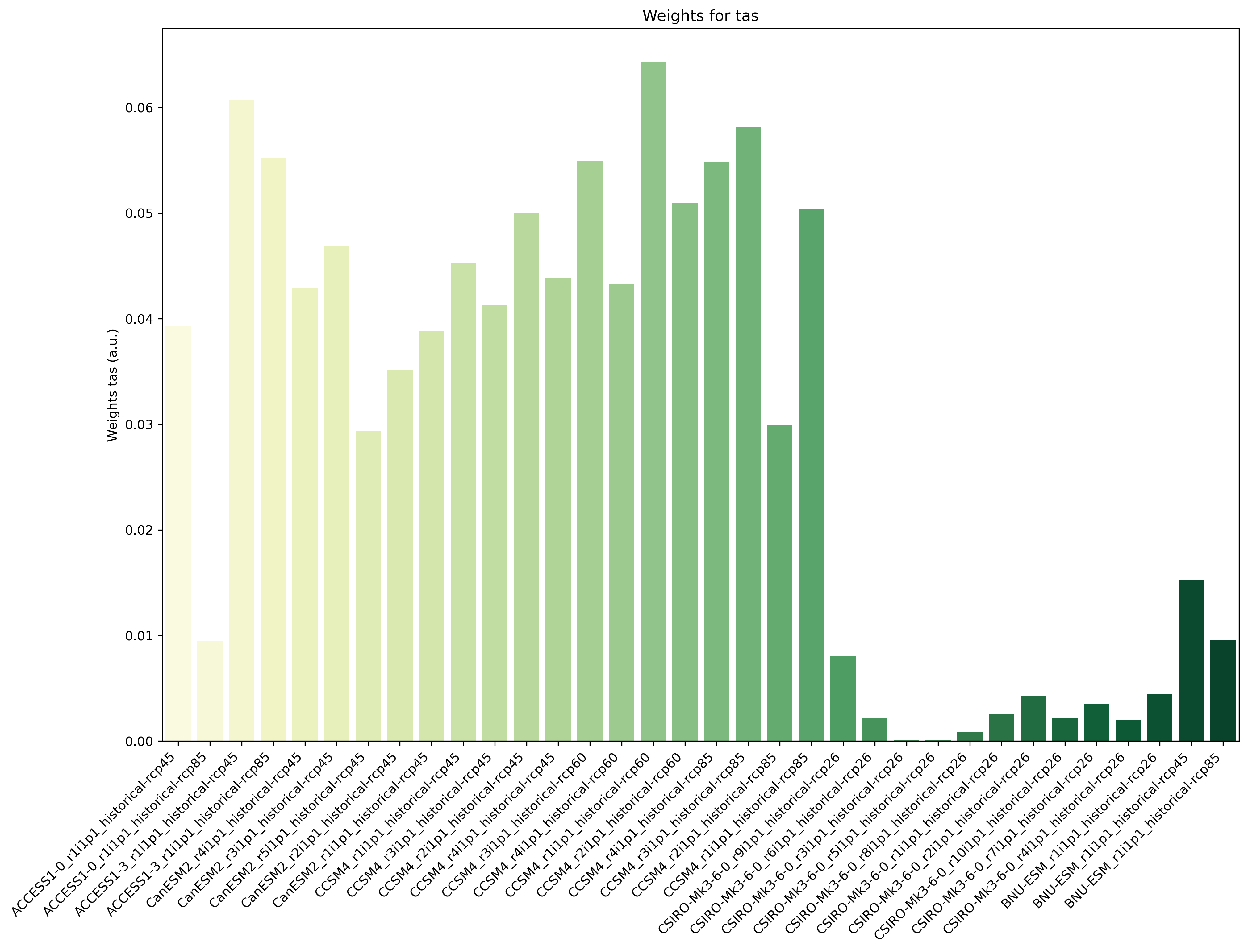
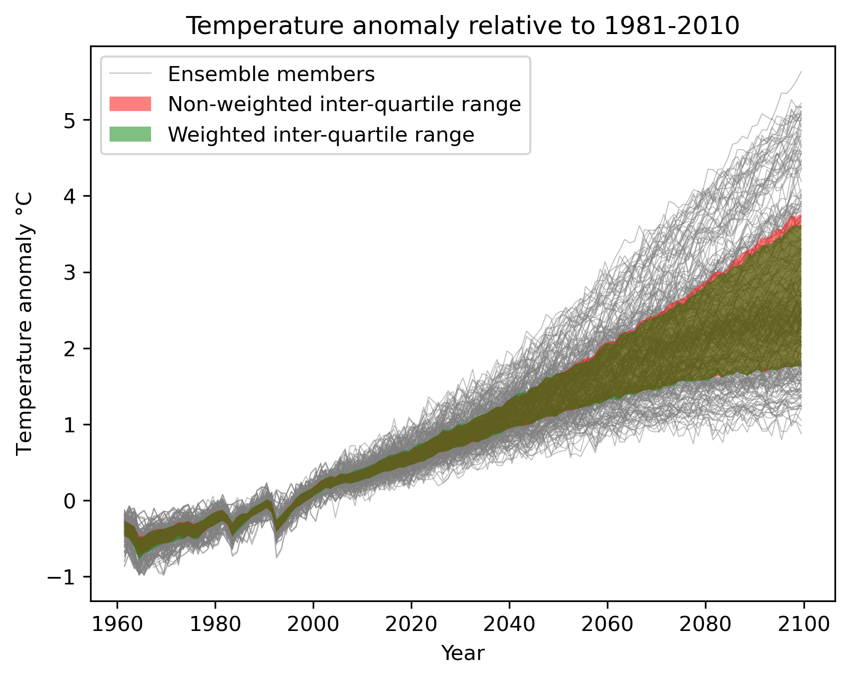
Fig. 7 Interquartile range of temperature anomalies relative to 1981-2010, weighted versus non-weighted.

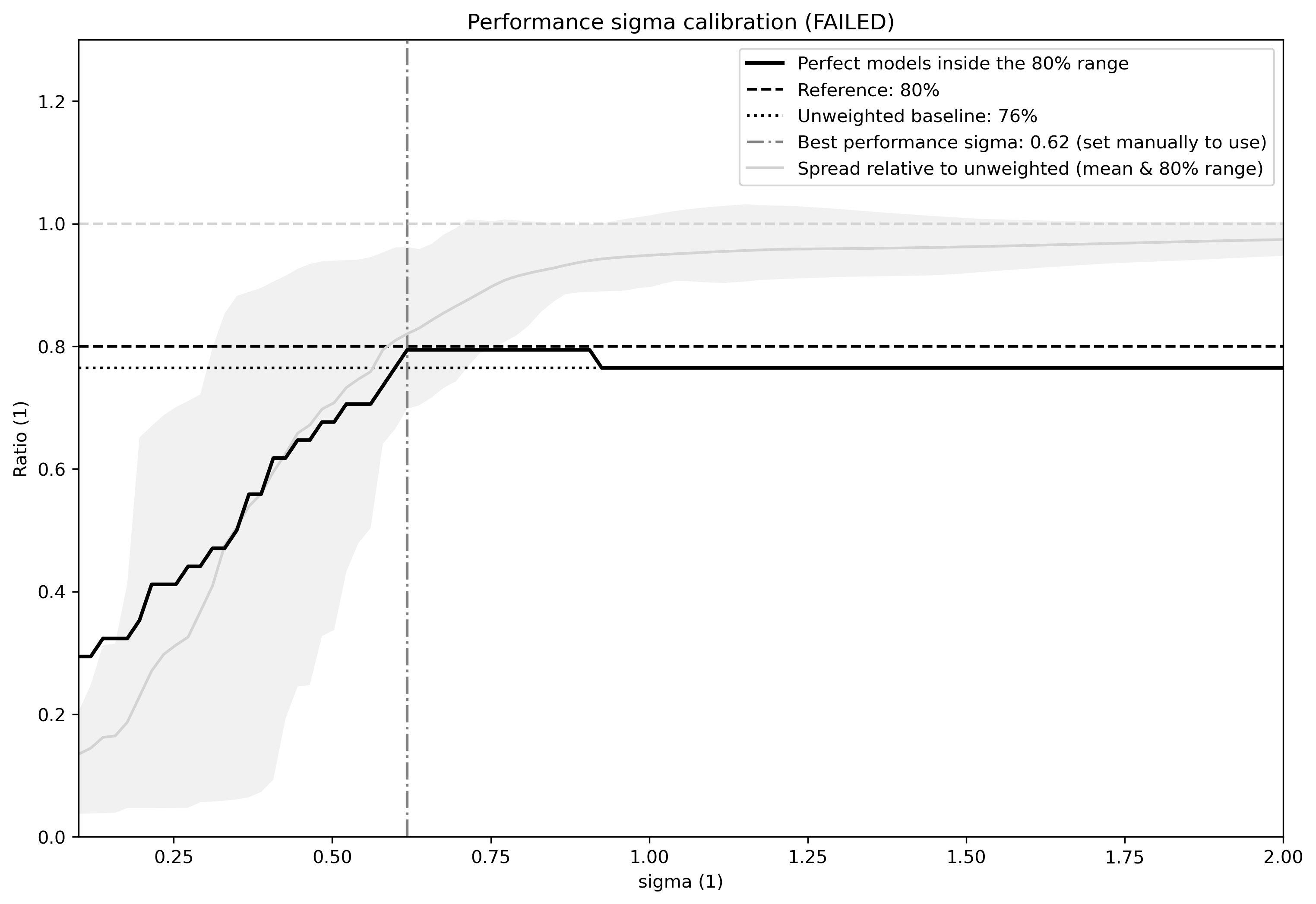
Fig. 8 Performance sigma calibration: The thick black line gives the reliability (c.f., weather forecast verification) which should reach at least 80%. The thick grey line gives the mean change in spread between the unweighted and weighted 80% ranges as an indication of the weighting strength (if it reaches 1, the weighting has no effect on uncertainty). The smallest sigma (i.e., strongest weighting) which is not overconfident (reliability >= 80%) is selected. If the test fails (like in this example) the smallest sigma which comes closest to 80% will be indicated in the legend (but NOT automatically selected).

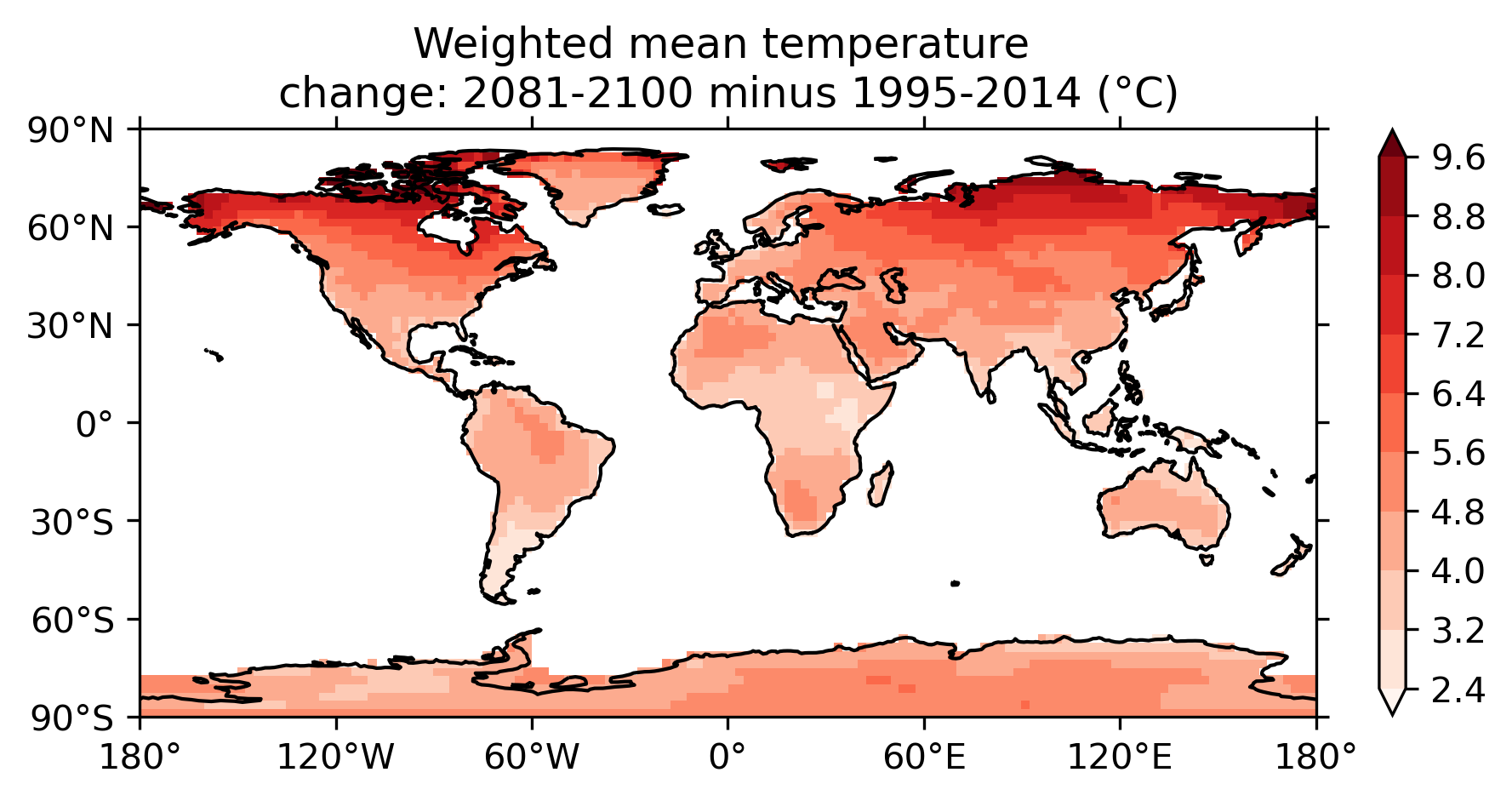
Fig. 9 Map of weighted mean temperature change 2081-2100 relative to 1995-2014