20. Sea ice
20.1. Overview
The sea ice diagnostics cover sea ice extent, concentration, and thickness. Work is underway to include other variables and processes in future releases of the ESMValTool. Current diagnostics include time series of Arctic and Antarctic sea ice area and extent (calculated as the total area (km2) of grid cells with sea ice concentrations (sic) of at least 15%). Also included are the seasonal cycle of sea ice extent, and polar stereographic contour and polar contour difference plots of Arctic and Antarctic sea ice concentration and sea ice thickness.
20.2. Available namelists and diagnostics
Namelists are stored in nml/
- namelist_SeaIce.xml
Diagnostics are stored in diag_scripts/
- SeaIce_tsline.ncl: time series line plots of total sea ice area and extent (accumulated) for northern and southern hemispheres with optional multi-model mean and standard deviation. One value is used per model per year, either annual mean or the mean value of a selected month.
- SeaIce_ancyc.ncl: as SeaIce_tsline.ncl, but for the annual cycle (multi-year monthly mean values).
- SeaIce_polcon.ncl: polar stereographic plots of sea ice concentration (= sea ice area fraction) and sea ice thickness for individual models or observational data sets, for Arctic and Antarctic regions with flexible paneling of the individual plots. The edges of sea ice extent can be highlighted via an optional red line.
- SeaIce_polcon_diff.ncl: polar stereographic plots of sea ice area concentration and thickness difference between individual models and reference data (e.g., an observational data set) for both Arctic and Antarctic with flexible paneling of the individual plots. All data are regridded to a common grid (1°x1°) before comparison.
20.3. User settings
User setting files (cfg files) are stored in nml/cfg_SeaIce/
- region: label of region to be plotted (“Arctic”, “Antarctic”); make sure to specify correct observational data for the selected region in the sea ice namelist.
- month: “A” = annual mean, “3” = March (Antarctic), “9” = September (Arctic)
- styleset: “CMIP5”, “DEFAULT”
- fill_pole_hole: fill observational hole at North Pole, default = False
- legend_outside: True: draw legend in an extra plot
Settings specific to SeaIce_polcon, SeaIce_polcon_diff, SeaIce_ancyc
- range_option: 0 = use each model’s whole time range as specified in namelist, 1 = use only intersection of all time ranges
Setting specific to SeaIce_tsline.ncl and SeaIce_ancyc.ncl
- multi_model_mean: plots multi-model mean and standard deviation (“y”, “n”)
- EMs_in_lg: create legend label for each individual ensemble member (True, False)
Settings specific to SeaIce_polcon.ncl and SeaIce_polcon_diff.ncl
- contour_extent: draw a red contour line for sic extent in polar stereographic plots (“y”, “n”)
- max_vert: max. number of rows on a panel page (vertical)
- max_hori: max. number of columns on a panel page (horizontal)
- max_lat: Antarctic plotted from 90°S up to this latitude
- min_lat: Arctic plotted from 90°N up to this latitude
- PanelTop: tune to get full title of uppermost row (1 = no top margin, default = 0.99)
Settings specific to SeaIce_polcon_diff.ncl
- ref_model: reference model, as specified in annotations; if this string is not found, the routine will print a list of valid strings before stopping
- dst_grid: path to destination grid file for Climate Date Operators (CDO), required by cdo_remapdis; e.g.: “./diag_scripts/aux/CDO/cdo_dst_grid_g010”
- grid_min: min. contour value (default = -1.0)
- grid_max: max. contour value (default = 1.0)
- grid_step: step between contours (default = 0.2)
- grid_center: value to center the color bar (default = 0.0)
20.4. Variables
- sic (sea ice, monthly mean, longitude latitude time)
- sit (sea ice, monthly mean, longitude latitude time)
20.5. Observations and reformat scripts
Note: (1) obs4mips data can be used directly without any preprocessing; (2) see headers of reformat scripts for non-obs4mips data for download instructions.
National Snow and Ice Data Center (NSIDC)
Reformat script: reformat_scripts/obs/reformat_obs_NSIDC.ncl
Hadley Centre Sea Ice and Sea Surface Temperature data set (HadISST)
Reformat script: reformat_scripts/obs/reformat_obs_HadISST.ncl
Pan-Arctic Ice Ocean Modelling and Assimilation System (PIOMAS)
Reformat script: reformat_scripts/obs/reformat_obs_PIOMAS.f90
20.6. References
- Bräu, M.: Sea-ice in decadal and long-term simulations with the Max Planck Institute Earth System Model, Bachelor thesis, LMU, 2013.
- Hübner, M.: Evaluation of Sea-ice in the Max Planck Institute Earth System Model, Bachelor thesis, LMU, 2013.
20.7. Example plots
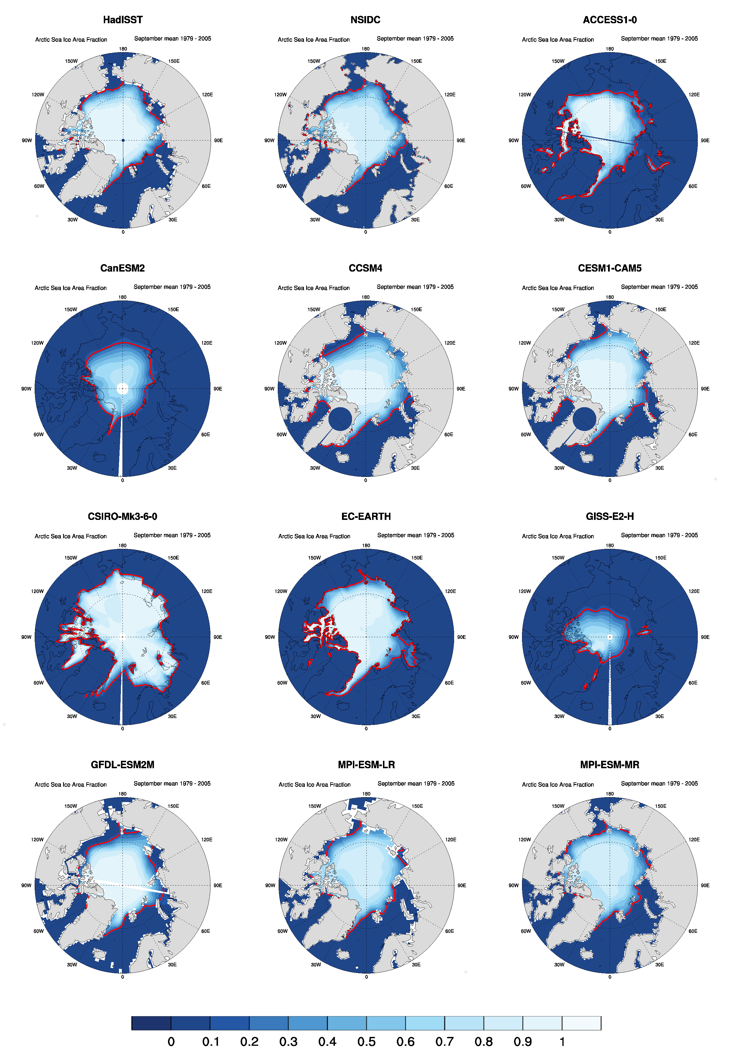
Figure 20.1 Polar-stereographic contour maps (Arctic) of sea ice concentration averaged over the period 1979-2005 from HadISST and NSIDC observations, as well as historical CMIP5 simulations from different Earth system models. The red line indicates the sea ice extent (i.e., sea ice concentration of 15%).

Figure 20.2 Polar-stereogrpahic projections (Antarctic) of the difference in sea ice concentration between historical CMIP5 simulations from different Earth system models and HadISST observations (1979-2005). Red (blue) colors indicate a positive (negative) bias of the respective model towards observations.
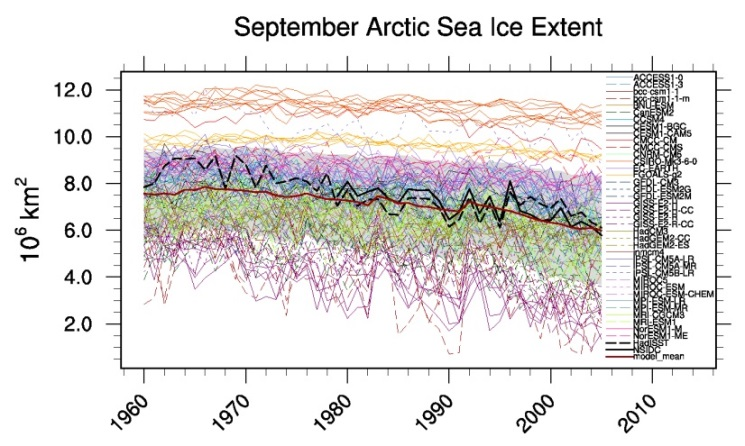
Figure 20.3 Timeseries (1960-2005) of September Arctic sea ice extent from different historical CMIP5 Earth system model simulations, and HadISST (black, dashed) and NSIDC (black, solid) observations. The thick red line represents the multi-model mean. Sea ice extent is the total area of all grid cells with a sea ice concentration of at least 15%.
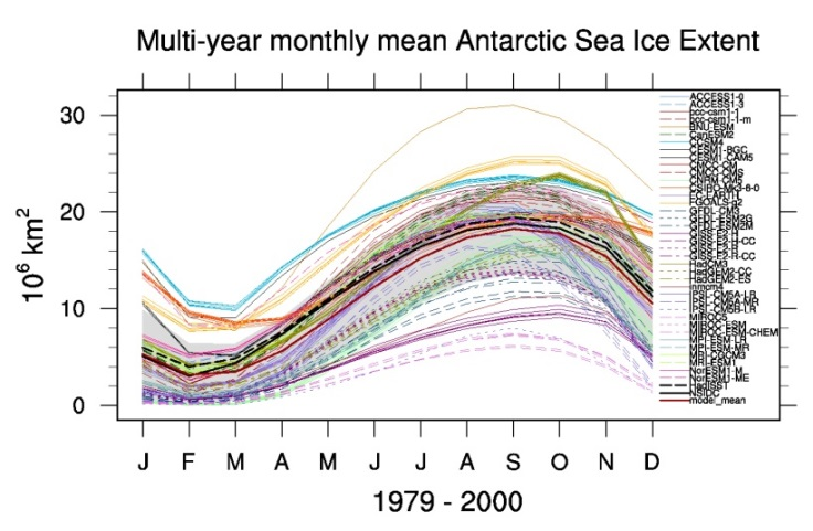
Figure 20.4 Same as Figure 20.3, but for the annual cycle of Antarctic sea ice extent.